![]()
DIA-NN
DIA-NN is an automated software suite for data-independent acquisition (DIA) proteomics data processing.
DIA-NN is built on the following principles:
- Reliability achieved via stringent statistical control
- Robustness achieved via flexible modelling of the data and automatic parameter selection
- Reproducibility promoted by thorough recording of all analysis steps
- Ease of use: high degree of automation, an analysis can be set up in several mouse clicks, no bioinformatics expertise required
- Powerful tuning options to enable unconventional experiments
- Scalability and speed: up to 1000 mass spec runs processed per hour
Download DIA-NN 2.5.1 Academia (limited functionality, for non-profit academic research): https://github.com/vdemichev/DiaNN/releases/tag/2.0.
DIA-NN 2.5.1 Enterprise (full functionality, for both Industry and Academia): contact Aptila Biotech aptila.bio or Speak with a Solutions Specialist | Thermo Fisher Scientific to purchase or obtain a trial license.
Table of Contents
Installation
Getting started with DIA-NN
Changing default settings
Raw data formats
Spectral library formats
Sequence databases
Output
Command interface
Analysis and visualisation
Automated pipelines
PTMs and peptidoforms
Fine tuning prediction models
Multiplexing using plexDIA
Editing spectral libraries
Custom decoys
Integration with other tools
Quantification
Speed optimisation
Incremental processing
InfinDIA
DDA
Basics of DIA data analysis
GUI settings reference
Command-line reference
Main output reference
Frequently asked questions
Troubleshooting
Key publications
Installation
On Windows, download and run the .msi file. It is recommended to install DIA-NN into the default folder suggested by the installer. If the Visual C++ runtime or .NET SDK are not already installed on the system, download and install vc_redist.x64.exe and the .NET SDK 8.0.407 installer, then reboot the PC.
On Linux, download and unpack the Linux .zip file. The Linux version of DIA-NN is built on Linux Mint 21.2, and the target system must provide glibc and other standard C/C++ libraries at versions equal to or newer than those on Linux Mint 21.2, plus .NET SDK 8.0-series (version 8.0.407 or later). Container images (Docker or Apptainer/Singularity) include all dependencies, removing any host-library requirements. To build a container, we recommend starting with the latest Debian Docker image; the included script make_docker.sh automates this process.
It is also possible to run DIA-NN on Linux using Wine 6.8 or later.
Getting Started with DIA-NN

If you are new to DIA proteomics, please take a look at the Basics of DIA data analysis.
A typical DIA-NN workflow has two stages: library preparation and data analysis. First, use DIA-NN to generate a predicted spectral library from the sequence database; this library can then be reused for all experiments involving the same organism. This first step is not necessary if one already has a suitable empirical spectral library (e.g. one generated by DIA-NN from a previous DIA experiment). Second, have DIA-NN analyse the raw data with the selected spectral library. Each step requires only a few mouse clicks.
Tip: DIA-NN includes a Wizard (accessible from the Pipeline panel toolbar) that guides step-by-step through setting up common analysis workflows, such as generating a predicted library, analysing raw data, creating empirical or calibration libraries, fine-tuning prediction models, or plexDIA analysis. The Wizard presents guided steps with context-appropriate defaults and recommendations, then automatically configures the settings. The Wizard effectively serves as a collection of interactive tutorials.
Predicted library generation:
- Click Add FASTA, add one or more sequence databases in UniProt format.
- In the Precursor ion generation panel, set Mode to Prediction from FASTA.
- (Optional) One can edit the Output library field. This field serves as a name template. In workflows that generate empirical DIA-based libraries, these are saved in Apache .parquet format as specified by Output library. For predicted library generation, however, the output file takes the
.predicted.speclibextension (DIA-NN’s own compact binary format for spectral libraries), with the name derived from the same template. - Click Run. DIA-NN’s log will be displayed in the Log panel. Library generation typically completes in under 2 minutes per million precursors on a modern 16-core desktop CPU.
Analysing with (any) spectral library:
- Click Spectral library and specify the library to use. This can be the .predicted.speclib file generated above, a .parquet library from a previous DIA-NN analysis, or a third-party predicted or empirical library in a compatible format (see below). Set Mode to Library search / Off.
- Click Add FASTA, add one or more sequence databases in UniProt format, corresponding to the spectral library (i.e. if the library contains human proteins, any human database is appropriate). If the library does not contain correct protein information (e.g. a third-party library), enable Reannotate to update the protein information for each precursor in the library.
- In the Input panel, click the + button next to Raw data files and select the raw data files (use Add .d for Bruker timsTOF .d folders).
- In the Output panel, adjust Main output. This is the name of the main output report generated by DIA-NN. It is also used by DIA-NN as the name template for any other report files it is going to generate (more about these below).
- Click Run. Note that DIA-NN will use the raw data to generate an empirical spectral library (file name specified by Output library).
If this is your first time running DIA-NN, we recommend reviewing the output on a small dataset that can be analysed in a couple of minutes. For this, download the raw data files (dia-PASEF 10ng.zip archive), empirical spectral library (K562-spin-column-lib.zip) and a FASTA database (human_canonical_uniprotkb_proteome_UP000005640_2023_12_16.fasta) from the Slice-PASEF benchmarks repository. When analysing this dataset, uncheck MBR (in the Algorithm panel) and Output library (in the Output panel).
Output:
-
The DIA-NN main report contains a list of all precursors (‘Precursor.Id’ column), with matched proteins (‘Protein.Group’ column) and quantities for both precursors and proteins (‘Precursor.Normalised’ and ‘PG.MaxLFQ’, respectively), for each run in the experiment. The report is in .parquet format – a compact compressed tabular format that can be accessed with the R
arrowor Pythonpolarspackages in automated fashion. One can also view the report and perform visualisation and statistical analysis (such as PCA, DA testing or GSEA) using the Analyse mode of the GUI. -
To quickly inspect protein quantities using software such as MS Excel, DIA-NN generates ready-to-use .pg_matrix.tsv and .unique_genes_matrix.tsv tab-separated tables. DIA-NN’s Analyse mode also allows to filter the main report and export quantitative matrices.
Changing default settings
LC-MS-specific parameters. For publication-ready/production-ready analyses, it is preferable to adjust the mass accuracies and the scan window used by DIA-NN. These parameters inform DIA-NN of the expected magnitude of mass deviations (mass accuracies) and the expected number of DIA cycles per average peptide elution time. By default, these are set to 0, meaning that DIA-NN will optimise them automatically for the first run in the experiment and then reuse the optimised settings for other runs. This optimisation is inherently noisy: even replicate injections may not produce identical results, and therefore the analysis results will depend on which run is first in the list. It is preferable to fix these three parameters to values known to be optimal for a particular LC-MS setup:
-
If the data were generated on timsTOF, set both MS1 accuracy (MS1 mass tolerance) and MS2 accuracy (MS/MS mass tolerance) to 15 (ppm). Note that these settings provide a ‘guidance’ to DIA-NN, the actual m/z window used to match theoretical m/z values to the (m/z, intensity) pairs in the raw data file will be specific to both the precursor and the raw data in the vicinity of its putative retention time.
-
If the data were generated on Orbitrap Astral, set MS1 accuracy to 4 and MS2 accuracy to 10. The MS1 accuracy setting here assumes 240k Orbitrap resolution, which is the optimal choice for the majority of experiments on Astral.
-
If the data were generated on TripleTOF 6600 or ZenoTOF, set both MS1 accuracy and MS2 accuracy to 20.
-
For Orbitrap instruments, the following table provides a good starting point for setting the mass accuracies:
| Orbitrap resolution | Accuracy (ppm) |
|---|---|
| 240k | 4 |
| 120k | 7 |
| 60k | 10 |
| 30k | 15 |
-
Set Scan window to the approximate number of DIA cycles during the elution time of an average peptide.
-
One can also optimise all parameters to achieve the best possible performance from the data. For this, run DIA-NN on several representative runs (best to use any suitable empirical library, as this is the quickest) with Unrelated runs option checked and review the ‘Averaged recommended settings for this experiment’ values reported at the end of the log.
-
(Enterprise edition) When analysing human samples, enable Knowledge base (Algorithm panel).
How to interpret the rest of this guide. The preceding guidance covers the vast majority of standard DIA-NN workflows. However, DIA-NN also offers powerful tuning options for specialised or unconventional experiments. When starting with DIA-NN, we recommend first running it on a few representative datasets to become familiar with its operation, and then reviewing the rest of this guide to determine whether any of the recommendations apply to the applications of interest. The rest of this guide provides detailed recommendations for specialised workflows.
In general, we recommend the following:
-
Only change the default settings if (i) the change is recommended in the present guide, or (ii) there is a clear rationale for the change given a specific type of experiment not covered in this guide, or (iii) the goal is to investigate the performance of alternative settings compared to the default settings that have been tested already.
-
Examine DIA-NN’s log for warnings/errors. The warnings and errors are printed when they occur as well as at the end of the log, i.e. one can immediately see them once the DIA-NN analysis finishes. They are also displayed by the QC Dashboard in Analyse mode.
-
DIA-NN prints some comments on the settings used at the top of the log, it is best to examine these the first time particular settings are used, to see if there are any recommendations.
Raw data formats
DIA-NN supports the following raw data formats: Thermo .raw, Bruker .d, Sciex .wiff, .mzML and .dia (DIA-NN’s own format for storing spectra). Conversion from any supported format to .dia is possible (except for Slice/diagonal acquisitions on timsTOFs). When running on Linux (native builds, not Wine), only .d, .raw, .mzML and .dia data are supported.
For .wiff support, download and install ProteoWizard – choose the 64-bit version that supports vendor files. Then copy all .dll files whose names contain ‘Clearcore’ or ‘Sciex’ from the ProteoWizard folder to the DIA-NN installation folder (the one containing diann.exe, DIA-NN.exe and auxiliary DIA-NN files).
.mzML files should be centroided and contain data as spectra (e.g. SWATH/DIA) and not chromatograms.
Technology support
- DIA and SWATH are supported - Orbitrap Astral is supported - FAIMS with constant CV is supported - Acquisition schemes with overlapping windows are supported - Gas-phase fractionation is supported - Scanning SWATH and ZT Scan DIA are supported - dia-PASEF/py-diAID are supported - Slice-PASEF is supported - midia-PASEF is supported - Other diagonal PASEF methods are supported, however accuracy of quantification needs to be validated with benchmarks - multiplexing with non-isobaric tags and SILAC is supported - MSX-DIA is not supportedConversion
Many mass spec formats, including those few that are not supported by DIA-NN directly, can be converted to .mzML using the MSConvertGUI application from [ProteoWizard](http://proteowizard.sourceforge.net/download.html). This works for all supported formats except Bruker .d and SCIEX Scanning SWATH or ZT Scan DIA – these need to be accessed by DIA-NN directly. The following MSConvert settings must be used for conversion: Binary encoding precision: 32-bit, Write index: checked, all other options in the Options panel unchecked, Peak Picking specified as the first filter, with Algorithm set to Vendor.Spectral library formats
DIA-NN supports comma-separated (.csv), tab-separated (.tsv, .xls or .txt) or .parquet tables as spectral libraries, as well as .speclib (compact format used by DIA-NN). For vast majority of applications, only DIA-NN-generated spectral libraries (.parquet or .speclib) should be used.
In detail
Libraries in the PeakView format as well as libraries produced by FragPipe, TargetedFileConverter (part of OpenMS) are supported directly, however, compatibility should be verified for each combination of software version, settings, and raw data type. DIA-NN can convert any library it supports into its own .parquet format. For this, click **Spectral library** (**Input** panel), select the library to convert, select the **Output library** file name (**Output** panel), click **Run**. If there is a need to use a library in an uncommon or non-standard format, it may be helpful to convert it to DIA-NN's .parquet and then examine the resulting library (using DIA-NN's **Analyse** mode, the R `arrow` package, or the Python `polars` package) to verify that the contents appear as expected. All .tsv/.xls/.txt/.csv/.parquet libraries are just simple tables with human-readable data, and can be explored/edited, if necessary, using DIA-NN's **Analyse** mode, Excel or R/Python.Sequence databases
DIA-NN accepts sequence databases in uncompressed FASTA format. The UniProt format is fully supported. For sequence databases in other formats, DIA-NN will typically extract the correct protein sequence IDs, but may not correctly read the protein names, gene names, and protein descriptions. In such cases, we recommend using an R package such as seqinr or Biostrings to reformat the database in UniProt format.
Output
The Output panel specifies where the output should be saved as well as the file names for the main output report and (optionally) the output spectral library. DIA-NN uses these file names to derive the names of all of its output files. The following subsections describe the different types of DIA-NN output. Most workflows require only the main report (for analysis using DIA-NN’s Analyse mode or in R or Python – recommended) or the matrices (simplified output for MS Excel). When the generation of Matrices is enabled, DIA-NN also produces a .manifest.txt file with a brief description of the output files generated.
Main report
A text table in .parquet format containing precursor and protein IDs, along with extensive associated metadata. Please use DIA-NN's **Analyse** mode or the R `arrow` or Python `polars` packages to process. These are complementary: the **Analyse** mode allows to obtain biological insights in minutes, featuring publication-quality visuals and built-in optimisations for DIA proteomics data. It is therefore highly useful for initial data analyses. R/Python, on the other hand, allow for full automation and fully customisable outputs, and are therefore recommended for generating final conclusions and visualisations. Most column names are self-explanatory, and the full reference as well as guidance on how to filter the main report can be found in [Main output reference](#main-output-reference). The following keywords are used when naming columns: - **PG** means protein group - **GG** means gene group - **Quantity** means non-normalised quantity - **Normalised** means normalised quantity - **TopN** means normalised protein quantity calculated using the TopN method when the **Quantification strategy** is set to **Legacy (direct)**; using these is usually not recommended - **MaxLFQ** means normalised protein quantity calculated using QuantUMS (**Quantification strategy** set to one of **QuantUMS** modes) or the MaxLFQ (**Quantification strategy** set to **Legacy (direct)**) algorithm, using quantities in this column is recommended for most applications - **Global** refers to a global q-value, that is calculated for the entire experiment - **Lib** refers to the respective global q-value saved in the spectral library; when using **MBR**, **Lib** q-values will correspond to q-values in the empirical DIA-based lib created in the first pass of **MBR**Matrices
These contain normalised QuantUMS or MaxLFQ quantities for protein groups ('pg_matrix'), gene groups ('gg_matrix'), unique genes ('unique_genes_matrix'; i.e. genes identified and quantified using only proteotypic, that is gene-specific, peptides) as well as normalised quantities for precursors ('pr_matrix'). They are filtered at 1% FDR, using global q-values for protein groups and both global and run-specific q-values for precursors. Additional 5% run-specific protein-level FDR filter is applied to the protein matrices, use --matrix-spec-q to adjust it. Sometimes DIA-NN will report a zero as the best estimate for a precursor or protein quantity. Such zero quantities are omitted from protein/gene matrices. A site-level report and site quantification matrices are also generated when variable modifications are declared and the FASTA database is provided, see [PTMs and peptidoforms](#ptms-and-peptidoforms).Protein description
The .protein_description.tsv file is generated along with the Matrices and contains basic protein information known to DIA-NN (sequence IDs, names, gene names, description, sequence).Stats report
Contains a number of QC metrics which can be used for data filtering, e.g. to exclude failed runs or as a readout for method optimisation. Note that the number of proteins reported here corresponds to the number of unique proteins (i.e. identified with proteotypic precursors) in a given run at 1% unique protein q-value. This number can be reproduced from the main report generated using precursor FDR threshold of 50% and filtered using Protein.Q.Value <= 0.01 & Proteotypic == 1. The definition of 'protein' in this context depends on the **Protein inference** setting.PDF reports
Two PDF reports, one containing QC metrics for each acquisition, another with trends observed over the experiment. The PDF reports are generated automatically by the DIA-NN GUI, once DIA-NN completes processing the raw data and generates a report.Flexible reanalysis
The **Output** panel controls how DIA-NN handles .quant files. DIA-NN processes raw data in two phases. It first performs the computationally demanding part of the processing separately for each individual run and saves the identifications and quantitative information to a separate .quant file. Once all runs are processed, it collects the information from all .quant files and performs cross-run steps, such as global q-value calculation, protein inference, calculation of final quantities, and normalisation. This architecture enables flexible reanalysis. For example, one can stop the processing at any moment and then resume starting with the run that was stopped at. One can also remove some runs from the experiment, add extra runs, and quickly re-run the analysis without having to reprocess the runs already completed. These capabilities are enabled by the **Reuse .quant files** option. The .quant files are saved to/read from the **Temp/.dia dir** (or the same location as the raw files, if no temp folder is specified). When using this option, it is essential to ensure that the .quant files were generated with the exact same settings as applied in the current analysis, with the exception of **FDR**, **Threads**, **Detailed log**, **MBR**, **Cross-run normalisation**, **Quantification strategy** and **Library generation** – these settings can differ. It is possible to transfer .quant files to another computer and reuse them there without transferring the original raw files. Important: it is strongly recommended to only reuse .quant files when both mass accuracies and the scan window are fixed to specific values (non-zero), otherwise DIA-NN will perform optimisation of these yet again using the first run for which a .quant file has not been found.Note: the reports in .parquet format provide the full output information for any kind of downstream processing. The .tsv matrices are there to simplify the analysis when using MS Excel or similar software. The numbers of precursors and proteins reported in different types of output files might appear different due to different filtering used to generate those, please see the descriptions above. All the ‘matrices’ can be reproduced from the main .parquet report, if generated with precursor FDR set to 50%, using R or Python.
Overriding protein and gene names
By default, DIA-NN reads the following protein metadata from the FASTA database: protein sequence identifier (accession; e.g. P02768), protein name (e.g. ALBU_HUMAN), gene name (e.g. ALB) and the protein description. DIA-NN supports commands that allow changing how these are treated, cf. [Command-line reference](#command-line-reference): --ids-to-names, --tag-to-ids, --species-ids and --species-genes. For example, --ids-to-names will result in Genes.MaxLFQ.Unique output column representing protein ID quantities obtained using protein ID-specific peptides. The other options can be useful for multi-species or entrapment benchmarking.Command interface
DIA-NN provides a graphical user interface (GUI) that invokes an underlying command-line tool (diann.exe, diann-linux or a container). The command-line tool can also be used separately, e.g. as part of custom automated processing pipelines. Further, even when using the GUI, one can pass options/commands to the command-line tool via the Additional options text field. All these options start with a double dash -- followed by the option name and, if applicable, some parameters to be set. Any option prefixed with -- in this guide should be entered in the Additional options text field. Some useful options are mentioned throughout this guide, and the full reference is provided in Command-line reference.
When the GUI launches the command-line tool, it prints in the Log panel the exact set of commands it used. To reproduce the behaviour observed when using the GUI (e.g. for automated analysis on a cluster), pass the same commands to the command-line tool directly.
diann.exe [commands]
Commands are processed in the order they are supplied, and with most commands this order can be arbitrary.
On Linux, some symbols have special meaning in the terminal, therefore, e.g. the semicolon ‘;’ (e.g. as part of –channels), the asterisk ‘*’ or the exclamation mark ‘!’ (e.g. in –cut) need to be preceded by a backslash on Linux for correct behaviour.
For convenience, as well as for handling experiments consisting of thousands of files, some of the options/commands can be stored in a config file. For this, create a text file with any extension, say, diann_config.cfg, type in any commands supported by DIA-NN in there, and then reference this file with –cfg diann_config.cfg (in the Additional options text field or in the command used to invoke the diann.exe/diann-linux command-line tool).
Analysis and visualisation
DIA-NN offers several tools for analysing, visualising, and interpreting proteomics results.
DIA-NN Analyse. Click Analyse in the Pipeline panel toolbar to open the Report Window, a comprehensive post-processing, analysis, and visualisation environment for DIA-NN output. The Analyse functionality requires a DIA-NN main report (.parquet) to be present. The Report Window provides six tabs, described below.
Experiment Design
The **Experiment Design** tab lets one assign experimental conditions and metadata to runs. This step is a prerequisite for differential expression and pathway analysis. * **Auto-detect**: Automatically parses run file names to populate condition columns. Useful when file-naming conventions encode experimental variables. * **Add Column**: Adds a new metadata column (of type "factor" or "characteristic") that one can fill in manually. * **Import / Export**: Import metadata from a tab-separated table or SDRF file; paste metadata from a spreadsheet; export the current design as TSV or SDRF for use in external tools. * **Cell editing**: Click any cell in the design table to edit its value directly. Right-click for batch operations (fill down, fill selection, clear). Column headers offer a context menu for renaming, changing the column type, sorting, splitting, merging, duplicating, or removing columns. * **Column type classification**: Each metadata column is automatically classified as **factor** (2-12 unique values), **continuous** (>=3 unique values, all numeric), or **characteristic** (everything else – 0-1 unique values or >=13 unique values). Only factor and continuous columns appear in analysis controls (conditions, covariates, PCA colour-by, heatmap annotations, etc.); characteristic columns are display-only. * **Undo / Redo**: All design changes can be undone and redone. * **Validation**: A panel above the table warns about potential issues such as conditions with only a single replicate.QC Dashboard
The **QC Dashboard** tab displays quality-control metrics for the experiment. * **Cross-run summary** (default view): a number of interactive chart panels, including identified protein groups and precursors per run, MS1 area and RT-deviation distributions, normalisation factor trends, retention time, ion mobility, and FWHM distributions, chromatographic profiles, and overall quantification quality. * **Per-run diagnostics**: Select an individual run to see a number of diagnostic plots, including RT, m/z, and charge-state distributions; 2-D heatmaps of RT vs predicted RT, IM vs m/z, FWHM vs RT, normalisation factor vs RT, and mass-accuracy (ppm) vs RT and vs m/z for both MS1 and MS2. * **Run selector**: Switch between the all-runs summary and any individual run. * **Colour by**: Colour the summary plots by any experiment design column, making it easy to spot batch effects or condition-specific trends. * **PDF export**: Export the current dashboard view to a multi-page PDF. * **Info buttons**: Each plot panel includes an ⓘ button that expands a short educational description of the metric.Filter
The **Filter** tab provides data-level filtering controls that are applied before any analysis on the next (Interpret) tab. * **Data Pipeline**: - Auto-filters are seeded on first use: `Q.Value <= 0.01` and `Global.PG.Q.Value <= 0.01` (plus channel-specific q-value filters for plexDIA data). These can be removed if needed. - **+ Filter**: Add custom filter expressions using column names and comparison operators (e.g. `PG.MaxLFQ > 0`). - **+ Column**: Add computed columns using expressions (e.g. `LOG2(PG.MaxLFQ) * 2`). - **Reset Pipeline**: Clears all user-added operations and re-seeds the default auto-filters. * **Run Filter**: - Exclude runs by minimum/maximum precursor or protein-group count. - Exclude runs by metadata column values (categorical selection or numeric range). - Exclude runs with median empirical quantification quality below a threshold (full dataset or top-10 protein groups). * **Apply & Rerun**: After adjusting filters, click this button (visible once an analysis has been run) to jump back to the Interpret tab and re-execute the current analysis with the updated filters.Interpret
The **Interpret** tab provides statistical analysis and interactive visualisation tools. It covers differential testing, principal component and factor analysis, pathway enrichment, and protein-level inspection including sequence coverage and regulation of individual precursors. The analysis results are exportable as both text tables and vector/raster graphics. DIA-NN automatically generates a description of all Methods used to produce the analysis. For advanced applications, the user is provided with a JavaScript sandbox with code to reproduce or modify the analysis. The tab is divided into a **sidebar** (configuration controls) and a **main area** (results, interactive plots, tables, and methods text). **Quantification level**. At the top of the sidebar, select the biological entity level for analysis. Available options depend on columns present in the DIA-NN report: * **Protein Groups** (`PG.MaxLFQ`) – default; analysis at the protein group level. * **Genes** (`Genes.MaxLFQ`) – gene-level quantities aggregated across all matching protein groups. * **Genes – Unique** (`Genes.MaxLFQ.Unique`) – gene-level quantities using only proteotypic (gene-specific) peptides. * **PTM Sites** – requires a `.site_report.parquet` next to the main report. When selected, a **localisation-confidence slider** (default >= 0.75) controls the minimum site-localisation probability. When **QuantUMS quality metrics** are detected in the data, two additional thresholds appear: a **per-sample quality** filter (minimum quality metric for each entity in each run) and an **average quality** filter (minimum average quality across runs). These provide an independent layer of quantitative quality control on top of standard FDR filtering and can be used to enhance the statistical analyses. **Analysis types**. Five analysis modes are available from the Analysis Type dropdown (Differential Abundance is selected by default): * **Table view**. A sortable, searchable table of all quantified entities. Each row shows the entity name, supporting precursor count, number of runs in which the entity was quantified, a colour-coded detection percentage, and summary statistics: mean, median, SD (on the log2 scale), and coefficient of variation (on the linear scale). A minimum coverage filter restricts the view to entities detected in a given proportion of runs. Clicking an entity name opens the **Entity Detail** overlay (see below). The quantitative matrix (entities x runs) can be exported as TSV, optionally with extra normalisation. * **Differential Abundance**. Identifies entities that are significantly up- or down-regulated between experimental conditions. Two comparison modes are supported: - *Pairwise (A vs B)*. Select a factor column and two conditions. Choose between **Welch's t-test** (default) and **Mann-Whitney U** for the per-entity test, or check one or more covariate columns to switch to a **linear model** (ordinary least squares per entity). An optional **interaction factor** enables full-factorial models: select a second factor and a **coefficient of interest** – Main effect (Factor A), Main effect (Factor B), or Interaction (A x B) – to test the corresponding term in the two-factor model. The **FDR threshold** and **|log2 FC| cutoff** can be adjusted after a run and update the display without recomputation. Results include a **volcano plot** (or MA plot), a results table, a fold-change histogram, and an auto-generated **expression heatmap** of top hits across all runs. Clicking a point on the volcano or a row in the table opens the Entity Detail overlay. - *ANOVA (all conditions)*. A one-way ANOVA F-test across all conditions in the selected factor. Results are shown as a **strip chart** of the top 20 significant entities (with individual data points coloured by condition) alongside an auto-generated expression heatmap. Options for **extra normalisation** (two-tier median equalisation that adapts to varying data completeness – a warning is shown when the available reference set is sparse, and normalisation is skipped if no reliable reference entities can be found) and **half-minimum imputation** (replaces each missing value with half the observed minimum across all runs) are available for both pairwise and ANOVA modes. A **minimum unique precursors** filter allows excluding entities with insufficient peptide evidence. * **PCA and factor analysis**. Principal component analysis of the quantification matrix. Two modes are available: - *Ubiquitous* (default): uses only entities quantified in every run, yielding a complete data matrix – no imputation is required. - *NA-tolerant O-ALS*: uses entities meeting a configurable minimum detection threshold (default 50 %), decomposed via alternating least squares on observed values only – missing values are neither imputed nor interpolated. **Metadata regression** ("Regress out") removes variance explained by selected design columns (e.g. batch, sex, instrument) before PCA by regressing them out per entity. Results include a **PCA scores scatter plot** (with configurable axes and colour-by metadata), a **scree chart** (variance explained per component), an expression heatmap for **top entities by loading magnitude**, annotated with PC loading values. The heatmap supports search, row/column clustering and configuring the colour-coded metadata rows. A link from PCA leads to **Pathway Analysis using PCA loadings** – see below. * **Correlation**. Pairwise Pearson correlation coefficients computed across all pairs of runs, displayed as a **clustered correlation heatmap** (hierarchical clustering with average linkage). A minimum detection threshold controls which entities are included. Useful for checking sample similarity, spotting outlier runs, and detecting batch effects. * **Pathway Analysis** offers two methods: - **CAMERA** (Wu and Smyth, 2012 – a competitive enrichment test that accounts for inter-gene correlations). Two analytical sources are supported: - *Condition-based*: ranks entities between two selected conditions using a configurable **gene ranking statistic**: fold change, t-statistic, or moderated t-statistic. An **Ignore empirical inter-gene correlations** option (enabled by default) uses a fixed inter-gene correlation of 0.05 (a commonly recommended CAMERA default) instead of estimating correlations empirically per gene set from the data. Optionally, **Covariates** can be specified. - *PCA loadings*: uses per-entity loading magnitudes from a previously completed PCA. This mode performs enrichment across all principal components simultaneously, presenting a **PC summary table** (which components carry significant pathway hits) with click-through to per-PC detail views. - **Gene set z-score testing** (Lee et al., 2008). An independent analysis that computes per-run mean z-scores for each gene set and tests for differential activity. Two comparison modes are supported: - *Pairwise (A vs B)*: select a factor and two conditions. Choose between Welch's t-test, Mann-Whitney U, or (with covariates checked) a linear model. - *ANOVA (all conditions)*: a one-way ANOVA F-test of mean z-scores across all conditions in the selected factor. An optional **interaction factor** enables full-factorial models with coefficient selection (Main effect (Factor A), Main effect (Factor B), or Interaction (A x B)), identical in semantics to the Differential Abundance interaction controls. A **Min. Detected per Sample** control (default 3) excludes a sample's activity score for a gene set when fewer than the threshold number of gene set member entities are detected in that sample, preventing noisy scores from influencing the test. **Extra normalisation** and **half-minimum imputation** operate on the entity-level expression matrix prior to z-score computation. **Annotation files** are loaded via a dialog with automatic format detection. Supported formats include WikiPathways GMT, GO Annotation (GAF/GPAD), QuickGO TSV, Reactome TSV, Reactome Complexes, HGNC, and generic 2-column or multi-column GMT. ID mapping files (NCBI gene_info for Entrez->Symbol, HGNC for UniProt<->Symbol) and GO definition files (.obo for human-readable term names) can also be loaded. The dialog includes download links organised by ID type. Loaded annotation files are cached across sessions. **Min set size** and **max set size** controls filter gene sets by the number of detected member genes (defaults: 3 and 500, respectively). Results include a **ranked results table** (gene set name, number of detected genes, enrichment score, direction, p-value, FDR). Clicking a gene set expands a **member panel** showing each member entity's rank and fold-change bar. Clicking a member opens the Entity Detail overlay. When WikiPathways or Reactome SVG maps are loaded, a **Map** button opens a **pathway map modal** with fold-change colour overlay; clicking a protein node in the map also opens Entity Detail. A **gene-set activity heatmap** is auto-generated after each pathway analysis, showing per-run mean z-scores for the top enriched sets. It supports search, row/column clustering, and click-through to per-gene expression heatmaps. **Entity Detail overlay**. Clicking any entity (from any analysis view, the table, or a heatmap) opens a detailed overlay with three tabs: * **Overview**: an abundance strip plot grouped by condition, a per-condition summary table (mean, SD, CV), and, when differential or pathway analysis has been run, the entity's log2 FC, p-value, and adjusted p-value. * **Precursors**: a summary table of all supporting precursors (with run coverage and mean abundance), a **precursor x run heatmap** with multi-factor condition colour bars, and a **concordance plot** showing precursor-level agreement (when differential or pathway analysis context is available). Note: the Precursors tab is hidden when viewing PTM site entities (Sites quantification mode). * **Sequence**: the full protein amino acid sequence with precursor mapping, fold-change colouring, and PTM annotation (requires a `.protein_description.tsv` alongside the report). In Site mode, the specific modification site is highlighted.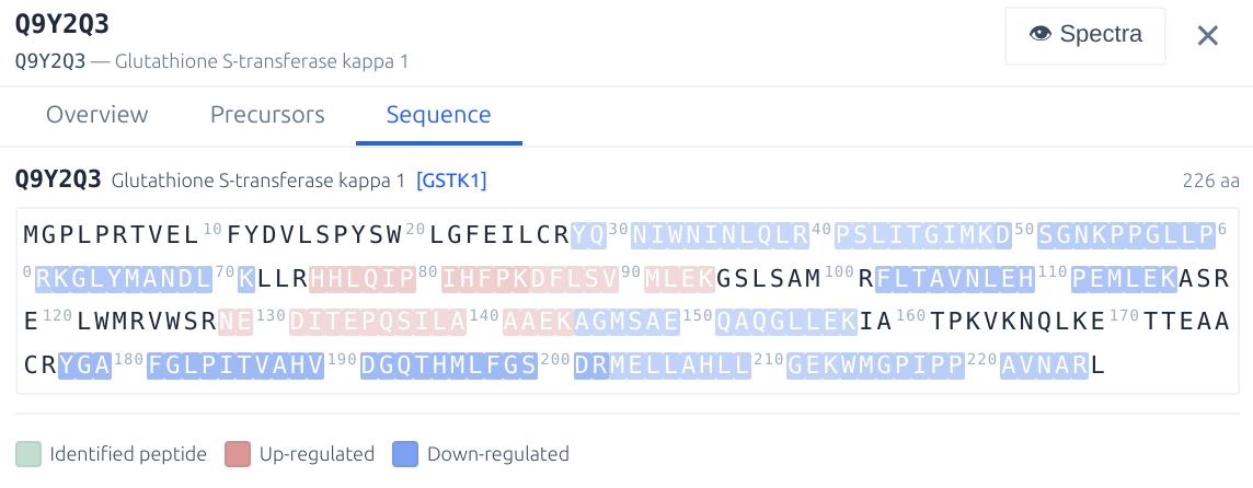
Spectra (XIC Viewer)
The **Spectra** tab provides the DIA-NN XIC Viewer. To use it, analyse the experiment with the **XICs** option enabled, then navigate to this tab. By default the **XICs** option will make DIA-NN extract chromatograms for the library fragment ions only and within 10s from the elution apex. Use `--xic [N]` to set the retention time window to N seconds (e.g. `--xic 60` extracts chromatograms within 60s of the apex) and --xic-theoretical-fr to extract all charge 1 and 2 y/b-series fragments, including those with common neutral losses. Note that using --xic-theoretical-fr, especially in combination with a large retention time window, might require a significant amount of disk space in the output folder. Regardless of experiment size, visualisation is effectively instantaneous. The XIC chart is interactive and displays the exact measured signals at each retention time on mouse hover. Currently, DIA-NN XIC Viewer does not support multiplexing.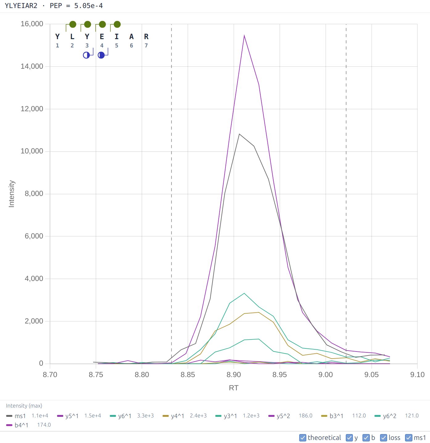
File (Parquet Browser)
The **File** tab provides a general-purpose viewer for .parquet files. Browse, filter, sort, and search the DIA-NN main report, site report, or any other .parquet table. This is convenient for quick checks on the raw DIA-NN outputs for specific peptides or proteins. Selected data can be exported as TSV (filtered subset or the complete table).Skyline. To visualise chromatograms/spectra in Skyline, analyse the experiment with MBR and a FASTA database specified, then click Skyline in the Pipeline panel toolbar. DIA-NN will automatically launch Skyline. Note the following limitations: this workflow does not currently support multiplexing, and it will not work with modifications in any format other than UniMod.
Automated pipelines
The Pipeline panel within the DIA-NN GUI allows multiple analysis steps to be combined into pipelines. Each pipeline step is a set of settings as displayed by the GUI. One can add steps to the pipeline, update existing steps, remove steps, move steps up/down, disable/enable (by toggling the checkbox) certain steps, and save/load pipelines. Individual pipeline steps can also be copy-pasted between different GUI tabs using the Copy and Paste buttons in the toolbar. It is recommended to assemble all analysis runs for a set of connected experiments into a single pipeline. One can also use DIA-NN pipelines to store configuration templates. When running a pipeline, each pipeline step is automatically saved as a separate one-step pipeline next to DIA-NN’s main report. Further, a pipeline can be run from the command line using the –pipeline command-line option of the GUI.
The Apply RegEx functionality is useful primarily for migration of pipelines between different machines. This field enables overwriting file paths in the pipeline using regular expression match-replace. The syntax is –regex “pattern to replace” “pattern to replace with”. Use –ignore-case to ignore letter case when matching. For example, the command
--ignore-case --regex "diann.exe" "C:/DIA-NN/2.0/diann.exe" --regex "C:/Out" "C:/Out/2.0" --regex "C:\\Out" "C:/Out/2.0" --regex "mass-acc-cal 30" "mass-acc-cal 100"
changes the DIA-NN binary file location to that of a specific version, adjusts some of the file paths accordingly and adjusts the calibration mass accuracy setting if specified anywhere in the pipeline.
Fine tuning prediction models
DIA-NN has the ability to fine-tune its retention time (RT) and ion mobility (IM) prediction models. This can substantially improve detection of modifications on which DIA-NN’s built-in models have not been trained.
Currently, the following modifications do not require any fine-tuning: UniMod:4 (C, carbamidomethylation), UniMod:35 (M, oxidation), UniMod:1 (N-term, acetylation), UniMod:21 (STY, phosphorylation), UniMod:121 (K, diglycine), UniMod:7 (NQ, deamidation). Fine-tuning can further improve detection for the following modifications: UniMod:888 (N-term, K, mTRAQ), UniMod:255 (N-term, K, dimethyl). Fine-tuning is likely to significantly boost detection of other modifications as well as unmodified cysteines.
Tuning. To fine-tune DIA-NN’s predictors, the only prerequisite is a spectral library (say, tune_lib.parquet; more on how to generate one below) containing peptides bearing the modifications of interest. Type the following in Additional options and click Run:
--tune-lib tune_lib.parquet
--tune-rt
--tune-im
If the library does not contain ion mobility information, omit –tune-im. If some modifications are not recognised, declare them using –mod. Tuning usually takes several minutes. DIA-NN will produce the following output files: tune_lib.dict.txt, tune_lib.rt.d0.pt (as well as .d1.pt and .d2.pt) and tune_lib.im.d0.pt (as well as .d1.pt and .d2.pt). The ‘d0’, ‘d1’ and ‘d2’ suffixes correspond to different model distillation levels (=sizes). These are automatically handled by DIA-NN. One can now generate predicted libraries using tuned models by supplying the following options to DIA-NN:
--tokens tune_lib.dict.txt
--rt-model tune_lib.rt.d0.pt
--im-model tune_lib.im.d0.pt
DIA-NN further allows to fine-tune also the fragmentation model, using –tune-fr. Here, however, the end result is highly sensitive to the quality of the library used for tuning, and the tuned model should always be verified to perform better than the base model. For fragmentation model tuning it makes sense to further test the effect of –tune-restrict-layers as well as different learning rates as set by –tune-lr.
Generating the tuning library. If there is no suitable tuning library, one can always generate it directly from DIA data. For this, select one or several ‘good’ (typically, largest size) runs that are expected to contain peptides with the modifications of interest. These runs can also come from some public data set. Make a predicted library with DIA-NN by specifying all modifications of interest as variable or fixed (including those the predictor has already been trained on, if they are expected to be present in the raw data). In vast majority of cases the max number of variable modifications can be set to 1-3, going higher is unlikely to be beneficial. Search the raw files using this predicted library in Proteoforms scoring mode, with Generate library selected, MBR disabled and Speed: RT/IM filtering set to Relaxed. If the search space is large, use the InfinDIA mode. If using DIA-NN to generate a tuning library for the fragmentation predictor, set Library generation (in the Algorithm panel) strategy to Full profiling.
If one uses a tuning library that is not an empirical library generated by DIA-NN’s lib-free search, and its RT & IM scales are significantly different from those produced by DIA-NN’s predictors, it is recommended to adjust the RT & IM values in the tuning library to approximately match DIA-NN’s (e.g. it is easy to do it if the tuning library contains some unmodified peptides, as those can be used for adjustment).
PTMs and peptidoforms
DIA-NN GUI features built-in definitions (via the modification selector’s quick-add toggles in the Precursor ion generation panel) for common modifications: N-term M excision, carbamidomethylation of cysteine, methionine oxidation, N-terminal protein acetylation, phosphorylation, ubiquitination (via the detection of remnant -GG adducts on lysines) and deamidation. Other modifications can also be selected from the full UniMod database as well as specified manually. Further, if convenient, modifications can be declared in Additional options as well, using –var-mod or –fixed-mod.
Distinguishing between peptidoforms bearing different sets of modifications is a non-trivial problem in DIA: without dedicated peptidoform scoring, the effective peptidoform FDR may reach 5-10 % for library-free analyses, depending on the dataset and modifications searched. DIA-NN implements a statistical target-decoy approach for peptidoform scoring, which is enabled by the Peptidoforms Scoring mode (Algorithm panel) and is also activated automatically whenever a variable modification is declared, via the GUI settings or the –var-mod command. The resulting peptidoform q-values reflect DIA-NN’s confidence in the correctness of the set of modifications reported for the peptide as well as the correctness of the amino acid sequence identified. These q-values, however, do not guarantee the absence of low mass shifts due to some amino acid substitutions or modifications such as deamidation (note that DDA does not guarantee this either). They are also not a replacement for dedicated channel-confidence scores, see Multiplexing using plexDIA.
Note: for purely peptidomics applications, such as a typical phosphoproteomics experiment, we recommend the Proteoforms Scoring mode, see GUI settings reference for details.
Further, DIA-NN features an algorithm which reports PTM localisation confidence estimates (as posterior probabilities for correct localisation of all variable PTM sites on the peptide as well as scores for individual sites), included in the .parquet output report. When matrix output is enabled and a FASTA database is provided, DIA-NN also produces a site-level report (.site_report.parquet). The site report contains the list of all occupied and unoccupied variable modification protein sites with the respective occupancy probabilities, for each precursor identification. Sites on a precursor are matched to sites on all proteins included in the respective protein group, in each case reported in a separate row of the site report. The entries in the site report can be matched to the main report and annotated with the information from it, as each row of the site report corresponds to a single row in the main report, defined by the combination of the run index, channel name and precursor library index.
For quick preliminary analyses using MS Excel or similar software, DIA-NN also generates ready-to-use quantitative matrices for the PTM sites, calculated using the Top 1 method, that is the highest intensity among precursors (passing certain confidence filters) with the site localised with the specified confidence (0.9 or 0.99, respectively) is used as the PTM quantity in the given run. Here, the sum of top 3 fragment intensities (ordered by their reference library intensities), multiplied by the precursor-specific normalisation factor, is used as the precursor intensity. One can also replace these with normalised MS1 apex intensities using –site-ms1-quant. The Top 1 algorithm is used here as it is likely the most robust against outliers and mislocalisation errors. However, whether or not this is indeed the best option needs to be investigated, which is currently challenging due to the lack of benchmarks with known ground truth (precision in LFQbench-type experiments is not a good proxy, as it does not model the possibly differential regulation of sites on the same peptide). It is recommended to rather rely on the site report, which is automatically recognised and loaded in DIA-NN’s Analyse mode but can also be accessed from R or Python, with matrices intended only for quick preliminary analyses with third-party software, as the site report provides one with full control over filtering as well as the quantification method. The matrices also are currently not being produced when multiplexing is used (–channels), in this case please rely on the site report.
In general, when looking for PTMs, we recommend the following:
-
Essential: the variable modifications one is looking for must be specified as variable (via the modification selector in the Precursor ion generation panel or the Additional options) both when generating an in silico predicted library and also when analysing the raw data using any predicted or empirical library.
-
Settings for phosphorylation: max 3 variable modifications, max 1 missed cleavage, phosphorylation is the only variable modification specified, precursor charge range 2-3; to reduce RAM usage, make sure that the precursor mass range specified (when generating a predicted library) is not wider than the precursor mass range selected for MS/MS by the DIA method; to speed up processing when using a predicted library, first generate a DIA-based library from a subset of experiment runs (e.g. 10+ best runs) and then analyse the whole dataset using this DIA-based library with MBR disabled.
-
When the above succeeds, also try max 2 missed cleavages.
-
When looking for PTMs other than phosphorylation, in the vast majority of cases best to use max 1 to 3 variable modifications and max 1 missed cleavage (unless the PTM modifies an amino acid that determines the cleavage specificity, in which case max 2 missed cleavages is recommended).
-
When not looking for PTMs, i.e. when the goal is relative protein quantification, enabling variable modifications typically does not yield higher proteomic depth. While it usually does not hurt either, it will make the processing slower.
The above recommendations aimed at limiting the search space can usually be disregarded when running InfinDIA.
Of note, when the ultimate goal is the identification of proteins, it is largely irrelevant if a modified peptide is misidentified, by being matched to a spectrum originating from a different peptidoform. Therefore, if the purpose of the experiment is to identify/quantify specific PTMs, amino acid substitutions or distinguish proteins with high sequence identity, then the Peptidoforms (or Proteoforms) scoring option is recommended, while in all other cases peptidoform scoring is typically fine to use but is not strictly necessary, and will usually lead to a somewhat slower processing and a slight decrease in identification numbers when using MBR.
Does DIA-NN need to recognise modifications in the spectral library?
Yes. If unknown modifications are detected in the library, DIA-NN will print a warning listing those, and it is strongly recommended to declare them using --mod. Note that DIA-NN already recognises many common modifications and can also load the whole UniMod database, see the --full-unimod option.Multiplexing using plexDIA
DIA-NN supports plexDIA, a technology that enables non-isobaric multiplexing (mTRAQ, dimethyl, SILAC) in combination with DIA. To analyse a plexDIA experiment, one needs an in silico predicted or empirical spectral library. DIA-NN then needs to be supplied with the following sets of commands, depending on the analysis scenario.
Scenario 1. The library is a regular label-free library (empirical or predicted), and multiplexing is achieved purely with isotopic labelling, i.e. without chemical labelling with tags such as mTRAQ or dimethyl. DIA-NN then needs the following options to be added to Additional options:
- –fixed-mod, to declare the base name for the channel labels and the associated amino acids
- –lib-fixed-mod, to in silico apply the modification declared with –fixed-mod to the library
- –channels, to declare the mass shifts for all the channels considered
- –original-mods, to prevent DIA-NN from converting the declared modifications to UniMod
Example for L/H SILAC labels on K and R:
--fixed-mod SILAC,0.0,KR,label
--lib-fixed-mod SILAC
--channels SILAC,L,KR,0:0; SILAC,H,KR,8.014199:10.008269
--original-mods
Note that in the above SILAC is declared as label, i.e. it is not supposed to change the retention time of the peptide. It is also a zero-mass label here, as it only serves to designate the amino acids that will be labelled. What the combination of –fixed-mod and –lib-fixed-mod does here is simply put (SILAC) after each K or R in the precursor id sequence, in the internal library representation used by DIA-NN. –channels then splits each library entry into two, one with masses 0 (K) and 0 (R) added upon each occurrence of K(SILAC) or R(SILAC) in the sequence, respectively, and another one with 8.014199 (K) and 10.008269 (R).
Scenario 2. The library is a regular label-free library (empirical or predicted), and multiplexing is achieved via chemical labelling with mTRAQ or any other label for which DIA-NN’s predictor has been fine-tuned (recommended: see Fine tuning prediction models).
Scenario 2: Step 1. Label the library in silico with mTRAQ (or the respective label) and run the deep learning predictor to adjust spectra/RTs/IMs. For this, run DIA-NN with the input library in the Spectral library field, an Output library specified, Mode set to Prediction from library, list of raw data files empty and the following options in Additional options:
--fixed-mod mTRAQ,140.0949630177,nK
--lib-fixed-mod mTRAQ
--channels mTRAQ,0,nK,0:0; mTRAQ,4,nK,4.0070994:4.0070994;mTRAQ,8,nK,8.0141988132:8.0141988132
--original-mods
Use the .predicted.speclib file with the name corresponding to the Output library as the spectral library for the next step.
Scenario 2: Step 2. Run DIA-NN with the following options:
--fixed-mod mTRAQ,140.0949630177,nK
--channels mTRAQ,0,nK,0:0; mTRAQ,4,nK,4.0070994:4.0070994;mTRAQ,8,nK,8.0141988132:8.0141988132
--original-mods
Note that –lib-fixed-mod is no longer necessary as the library generated in Step 1 already contains (mTRAQ) at the N-terminus and lysines of each peptide.
Scenario 3. The library is a regular label-free library (empirical or predicted), and multiplexing is achieved via chemical labelling with a label other than mTRAQ or a label for which DIA-NN has been fine-tuned. The reason this scenario is treated differently from Scenario 2 is that if DIA-NN’s in silico predictor has not been specifically trained for a label, the extra step to generate label-specific predictions is not necessary. Simply run DIA-NN as you would do in Scenario 1, except the –fixed-mod declaration will have a non-zero mass in this case and will not be a label. For example, for 5-channel dimethyl as described by Thielert et al:
--fixed-mod Dimethyl, 28.0313, nK
--lib-fixed-mod Dimethyl
--channels Dimethyl,0,nK,0:0; Dimethyl,2,nK,2.0126:2.0126; Dimethyl,4,nK,4.0251:4.0251; Dimethyl,6,nK,6.0377:6.0377; Dimethyl,8,nK,8.0444:8.0444
--original-mods
Note that Scenario 3 is relevant only for quick preliminary analyses, whereas Fine tuning prediction models should be used for any production-level work involving such chemical labels.
Scenario 4. The library is an empirical DIA library generated by DIA-NN from a multiplexed DIA dataset. For example, this could be a library generated by DIA-NN in the first pass of MBR. The Additional options will then be the same as in Scenario 1, Scenario 2: Step 2 or Scenario 3, except (important!) –lib-fixed-mod must not be supplied.
Scenario 5. The sample is a light sample with heavy spike-in proteins or peptides, that is only a small proportion of precursors should feature multiple channels. In this case, start with two unlabelled spectral libraries, one for the whole proteome, another for the spike-ins. Make sure that the RT and IM scales in those are similar and fragmentation information is likewise comparable – this will be the case if the libraries are predicted by DIA-NN. Using Editing spectral libraries make sure that (i) the whole proteome library does not contain precursors corresponding to spike-in peptides and (ii) the spike-in library has appropriate channel family tags applied to the precursor/peptide names. Combine the libraries in DIA-NN and proceed as in Scenario 3, except omit –lib-fixed-mod.
In all scenarios above, an extra option specifying the normalisation strategy must be included in Additional options. This can be either –channel-run-norm (pulsed SILAC, protein turnover) or –channel-spec-norm (multiplexing of independent samples). This is necessary as the raw data alone does not contain sufficient information for DIA-NN to infer the nature of the experiment.
Output. When analysing multiplexed data, the main report in .parquet format needs to be used for all downstream analyses. Note that PG.Q.Value and GG.Q.Value in the main report are channel-specific, when using multiplexing. The quantities PG.MaxLFQ, Genes.MaxLFQ and Genes.MaxLFQ.Unique are only channel-specific if (i) QuantUMS is used and (ii) either the report corresponds to the second pass of MBR or MBR is not used. The quantities must be channel-specific for any meaninful downstream analysis.
Channel confidence. DIA-NN estimates channel-confidence of identifications (expressed as Channel.Q.Value and PG.Q.Value) by searching an in silico generated ‘decoy’ channel and then comparing the numbers of identifications in this channel and cognate channels, at a given score threshold. The decoy channel generated is displayed by DIA-NN at the top of its log and can be overriden using –decoy-channel. Note that the channel confidence estimates obtained will be biased if the decoy channel turns out to be a poor model for the target channel-mismatched identifications. For example, in case of +0, +4 and +8 target channels, decoy channel +12 will result in conservative channel q-values if +8 is a carrier while +0 and +4 are single cells, and in optimistic channel q-values if +0 is the carrier. However, these fluctuations in accuracy of channel confidence estimation would typically still allow for quality quantification with any reasonable (0.01-0.05) q-value filters.
Note: QuantUMS quality metrics provide independent control for channel confidence and can be used in addition (recommended) or instead of channel-specific q-value filtering.
Editing spectral libraries
This section summarises operations on spectral libraries that can be helpful for certain specialised experiments.
DIA-NN itself can:
- Convert any spectral library compatible with it to .parquet format. For this, specify the input library in Spectral library field and click Run (Raw field must be empty). Note that analysis with a converted library may produce results that are not identical to the analysis with the original library, e.g. due to real number precision limits, DIA-NN discarding decoy peptides that match target sequences, DIA-NN adjusting protein annotation of decoy peptides or in general changing the order in which proteins are listed.
- Merge several .parquet or .tsv libraries, for this use multiple –lib commands in Additional options. Note the warnings printed by DIA-NN.
- Replace the spectra, RTs and IMs in the library with predicted ones using deep learning. Note –dl-no-fr, –dl-no-rt and –dl-no-im that allow to control what gets replaced.
- Apply fixed modifications to the library using –lib-fixed-mod. This changes peptide names and, if the modification has non-zero mass, also precursor and fragment masses.
Using R or Python, one can further:
- Edit .tsv or .parquet libraries in arbitrary way, including filtering, editing RTs and IMs, changing peptide sequences, adding ‘faux’ modifications (e.g. pasting ‘(SILAC)’ after specific amino acids, to be later on used with –channels) and editing modification names, adding decoy peptides, marking fragments that should not be used for quantification, editing proteotypicity information for precursors, adjusting how proteins are annotated.
- Combine .tsv or .parquet libraries, here it is important to make sure that there are no duplicate precursors in the resulting library.
Note that whenever a .parquet library is being edited, when saving to disk (i) all floating point columns must have the FLOAT parquet type and (ii) all integer or boolean columns must have the INT64 parquet type, (iii) the original order in which fragments of a precursor were listed must be maintained. Below is the sample code that edits library sequences to paste-in (SILAC) tags after K or R as well as changes the retention time scale:
library(arrow)

lib <- read_parquet("lib.parquet", as_data_frame=F, mmap=F) # Load the library
schema <- arrow::schema(lib) # Schema records original column types
lib <- as.data.frame(lib) # Cast to base R data frame

lib$Modified.Sequence <- gsub("([KR])", "\1(SILAC)", lib$Modified.Sequence) # Edit modified sequences
lib$RT[lib$RT > 0.0] <- lib$RT[lib$RT > 0.0] * 2.0 # Edit RT scale

write_parquet(as_arrow_table(lib,schema=schema), "edited_lib.parquet") # Restore column types and save to .parquet
Custom decoys
This section describes DIA-NN’s ability to customise its decoy models. This capability is not needed for the vast majority of experiments. However, this functionality is essential for correct handling of data wherein a substantial proportion of peptides incorporates specific sequence patterns, and, to our knowledge, is a unique feature of DIA-NN.
DIA-NN implements two main approaches to decoy generation based on a target peptide: (i) shuffling of the residues using a particular algorithm and (ii) mutation of a single residue. DIA-NN has the following decoy generation parameters, which it will attempt to abide by whenever possible and will only ignore if it cannot generate the decoy otherwise:
- –dg-keep-nterm [N] do not change the first N residues, default N = 1
- –dg-keep-cterm [N] do not change the last N residues, default N = 1
- –dg-min-shuffle [X] aim for any fragment mass shift introduced by shuffling to exceed X in absolute value, default 5.0
- –dg-min-mut [X] aim for the precursor mass shift during mutation to be at least X in absolute value, default 15.0
- –dg-max-mut [X] aim for the precursor mass shift during mutation not to exceed X in absolute value, default 50.0
In particular, the options restricting N-term and C-term residue changes are essential in a situation when the target peptides are e.g. synthetic peptides that all share several N-term or C-term residues.
Integration with other tools
This is a quick reference section for third-party software developers.
It is possible to supply DIA-NN with decoy peptide queries in the spectral library (.parquet) along with the target peptides. This allows DIA-NN to use its MBR-optimised algorithm to correctly control FDR with empirical libraries generated by third-party software. For this, the third-party software needs to generate its libraries in DIA-NN-compatible .parquet format: (i) include all the columns except Signature, which must not be present; (ii) the column ‘Flags’ sets 1 « 0 for all rows and 1 « 4 for the first fragment per precursor; (iii) Source.Id is the target precursor by mutation of which the decoy has been obtained, or, if not available, an appropriately matched (AA composition, charge, protein) arbitrary target precursor. Ideally, the libraries should contain:
-
A proportion of decoy peptides, corresponding the to q-value filtering applied when generating the library. DIA-NN will search these decoys in addition to the regular decoys it generates.
-
Q-values for all entries, target and decoy, for both precursors and protein groups. In case decoys are not provided, including q-values may, in most cases, largely ensure correct FDR control by itself, if the library if filtered at precursor q-value <= 0.01 or below.
The numeric columns in DIA-NN’s .parquet libraries are of types INT64 and FLOAT, other types should not be used.
For third-party downstream tools, it may be useful to have DIA-NN also export the decoy identifications using –report-decoys.
Quantification
DIA-NN implements Legacy (direct) and QuantUMS quantification modes. The default QuantUMS (precision) is recommended in most cases. QuantUMS enables machine learning-optimised relative quantification of precursors and proteins, maximising precision while substantially reducing ratio compression, see Key publications. DIA-NN 2.0 has a much improved set of QuantUMS algorithms, compared to our original preprint.
Note that if an empirical library is used for analysis, one can quickly generate reports corresponding to different quantification modes with Reuse .quant files. This can also be done just for a subset of raw files, e.g. to exclude blanks.
We have observed that:
-
QuantUMS performance is largely unchanged regardless of the experiment size, i.e. it is suitable for large experiments.
-
QuantUMS works well also on experiments which include very different sample amounts (tested with 10x range across different samples). Note, however, that in this case the optimisation of QuantUMS parameters, automatically performed by DIA-NN, largely tunes the algorithm to quantify most accurately ‘representative’ identifications, i.e. if the experiment consists of 10 bulk runs and 10 single cell runs, optimisation will turn out to be optimal for bulk runs.
-
QuantUMS has been tested with sub 2-minute to over 90 minute gradients and with both bulk and single cell-like samples.
-
QuantUMS is particularly beneficial for Orbitrap Astral data due to the high quality of its MS1 spectra.
Below are some recommendations for the use of QuantUMS.
High-accuracy. Use the high-accuracy mode when it is desirable to minimise the ratio compression at the cost of precision. Note that while it does a very good job at this in most cases, DIA-NN still cannot completely eliminate ratio compression for low-abundant precursors and proteins in challenging samples, e.g. when analysing nanogram amounts at 200-500 samples/day throughput. This is because many precursors in such cases lack any high-quality signal.
For large experiments, train QuantUMS on a subset of runs (e.g. 10 to 100 representative runs with medium to high numbers of identified precursors) and then quantify the whole experiment by reusing the QuantUMS parameters. For this, first run QuantUMS on a subset of runs, e.g. by selecting only those runs in Raw files window and checking Reuse .quant files. Alternatively, one can specifically instruct QuantUMS to train only on a range of raw files (by index, starting with 0) using –quant-train-runs first:last, e.g. –quant-train-runs 0:5 will perform training on identifications from the first 6 runs. A third option (not recommended) is to instruct DIA-NN to automatically select N runs (use N between 6 and 100) to train QuantUMS with –quant-sel-runs [N]. As output, a list of quantificaton parameters will be printed in the log, e.g.
Quantification parameters: 0.330076, 0.123932, 1.03485, 0.324712, 0.241882, 0.271245, 0.161143, 0.0203897, 0.019745, 0.0728814, 0.0574469, 0.0620889, 0.206804, 0.0761579, 0.0977414, 0.0613432
These parameters can be reused to skip training on the whole (large) experiment with –quant-params, e.g.
--quant-params 0.330076, 0.123932, 1.03485, 0.324712, 0.241882, 0.271245, 0.161143, 0.0203897, 0.019745, 0.0728814, 0.0574469, 0.0620889, 0.206804, 0.0761579, 0.0977414, 0.0613432
QuantUMS can be trained on replicate injections of the same sample: we have verified on a diverse set of LC-MS setups that such training results in near-optimal parameters even when trained on triplicates. Nevertheless, QuantUMS does require at least some degree of variation in the data. Even in replicate injections, some quantitative variation is always present due to fluctuations in instrument performance. Therefore, we recommend training QuantUMS on subsets of runs that include at least some non-replicates. In practice, this is rarely a limitation, as most experiments encompass sufficient biological or technical variation.
The optimality of specific parameters for a particular experiment depends on the LC-MS settings (gradient, acc/ramp times, acquisition scheme) and the general type of sample (e.g. whole-cell vs AP-MS). It is likely OK to even reuse QuantUMS parameters between experiments with the same LC-MS settings and general sample types, so long as the training is performed on data corresponding to the same or larger sample amounts and the ‘instrument sensitivity’ was at its highest when the training data were acquired. The opposite is not recommended.
Filtering. One of the benefits of QuantUMS is that it provides ‘quality’ metrics for each quantity it reports. We recommend using both Quantity.Quality and PG.MaxLFQ.Quality for filtering. In most cases, it makes sense to apply a relatively strict filter on the average quality metric for the analyte and much less strict filter on its run-specific quality metric. The average filter may increase numbers of DE analytes at a given FDR, as less analytes under consideration mean less strict multiple testing correction. The run-specific filter is best chosen to retain the vast majority of identifications, while eliminating the ones with very low quality quantities. The (Enterprise-only) MaxLFQ.Empirical.Quality protein-level metrics integrate both the LC-MS data quality and the concordance of precursor regulation within a protein into a single quality score. A low empirical quality score implies lack of overwhelming support for the calculated protein quantity across multiple matched precursors. A high score, however, indicates the likelihood but does not guarantee concordant regulation. The MaxLFQ.Empirical.Quality may be used in addition or instead of MaxLFQ.Quality for filtering.
Legacy mode is to be used in the following cases:
-
Always use the legacy mode when benchmarking LC-MS (settings). This is due to the fact that QuantUMS does not have the objective to minimise CV values, rather its goal is to achieve a good balance between precision and accuracy. This balance may differ significantly between different LC-MS settings, and using a single metric such as the median coefficient of variation (CV) reflects only part of this balance. Therefore, for experiments where QuantUMS simply decides to emphasise precision to a greater extent, CV values will appear better.
-
You would like to use the Top N protein quantities (normally not recommended) instead of the built-in QuantUMS MaxLFQ-like algorithm. QuantUMS precursor quantities are currently not intended to be used for Top N, as QuantUMS is inherently a ‘relative quantification’ method, whereas Top N effectively implies comparing quantities of different precursor ion species.
-
For the same reason, use the legacy mode for IBAQ.
-
In all the above (rare) cases where comparisons between quantities of different precursor species are performed (= absolute quantification is important) and the legacy mode is therefore appropriate, also consider just using the raw fragment quantities (at the apex), reported by DIA-NN when using –export-quant, e.g. summing the first 3 fragments may in some cases be better than using the legacy quantities. The normalisation factors calculated by DIA-NN in any mode can also be applied to the raw fragment quantities. Further, in all such scenarios one may want to use the Top N approach (with N between 1 and 3) for any kind of precursor quantities aggregation (e.g. protein quant) rather than MaxLFQ (because if MaxLFQ were appropriate, would be better to use QuantUMS).
Zero quantities. Any of the quantities produced by DIA-NN may be zero. A zero quantity should be interpreted as indicating that the analyte concentration is below the limit of reliable quantification. If the data needs to be log-transformed, these zeroes can be replaced with NA values. We prefer to report zeroes rather than change the algorithm to output noise or NAs, as zeroes provide extra information which may be of value for some downstream workflows.
Synchro-PASEF. When analysing Synchro-PASEF data, use –quant-tims-sum, which makes DIA-NN quantify each fragment in each DIA cycle by summing the signals recorded in all cognate frames within the cycle. While this is expected to provide adequate quantification performance, it has not been established whether minor IM calibration drift between acquisitions introduces batch effects in Synchro-PASEF data; certainty will require dedicated benchmarks.
Normalisation. DIA-NN implements different normalisation modes. Normalisation can correct for different amounts of input material and sample losses. The RT-dependent normalisation further corrects for factors that differentially affect peptides depending on their hydrophobicity (reflected by their RT), i.e. some types of sample preparation losses, including desalting, as well as possibly also fluctuations in the ion source performance. There are multiple examples of experiments where RT-dependent normalisation has a major positive effect on quantitative performance and no known cases where it is substantially detrimental.
Limitations of normalisation. In general, any kind of generic normalisation in proteomics only makes sense under the following assumption: when only considering ‘biological’ variability of interest, most of the peptides are not differentially abundant, or the numbers of upregulated / downregulated (in comparison to experiment-wide averages) peptides in each sample are about the same. This assumption often is not strictly satisfied. Reasons include the non-linear dynamic range of the LC-MS system and fundamental biological differences between samples (e.g., ideally, different normalisation factors may need to be applied to cytosilic, plasma membrane or chromatin proteins, when comparing two single cells of different sizes). However, in many ‘typical’ proteomics experiments the normalisation algorithms implemented by DIA-NN work very well still. Nevertheless, it is recommended to not include blanks/failed runs in quantitative analyses, i.e. if blanks are processed to monitor carryover, one can always process them separately with the emprical library produced by DIA-NN based on the experiment. Further, best to avoid a situation when the majority of precursors in a particular sample are not detectable in most other samples, e.g. not to include bulk runs in the quantitative analyses of single cell samples (but can absolutely use them to generate the empirical library).
Disabling normalisation. Given the above, there are scenarios (e.g. AP-MS, any kind of protein fractionation, time-series tracking isotopic label incorporation) when it may be desirable to apply custom normalisation that takes into account the nature of the experiment. In this case, we suggest either (i) disabling the normalisation in DIA-NN – one can still use MaxLFQ quantities in this case or (ii) keeping normalisation set to RT-dependent and applying custom normalisation on top of that, to benefit from DIA-NN correcting for any RT-dependent perturbations. The latter makes sense if there is still a considerable fraction of peptides that are shared between the samples.
Fold-changes. Given that normalisation is never 100% perfect, it is usually recommended to incorporate fold-change cutoffs in any differential expression (DE) analysis. These do not need to be particularly large in magnitude, but should at least exceed the expected error in normalisation, e.g. when treating a cell line with drug compounds that have minor effects on the cells, even 10% fold-change cutoff may be appropriate. Fold-change cutoffs have also a further benefit of substantially reducing the FDR. Important: fold-change cutoffs must be applied after adjusting the p-values via multiple testing correction, not before.
Detecting normalisation errors. Errors in normalisation may be easy to identify. For example, the number of points with positive and negative fold-changes on a volcano plot should almost always be balanced. Indeed, one or several pathways may be upregulated in one condition compared to another, but if most pathways seem to be upregulated, it would mean most proteins are upregulated, implying that the dataset has not been correctly normalised. This check does not apply to certain specialised workflows such as AP-MS. In Analyse mode, the DIA-NN GUI shows a fold change histogram for differential abundance (DA) analyses, to provide a basic normalisation quality control.
A simple normalisation test can further be carried in R or Python. For any two samples
- Calculate log2 fold-change of each analyte (precursor or protein) between the samples.
- Plot the histogram of the above log2 fold-changes.
- Indicate the median and half sample mode (use hsm() function of the modeest R package) on the histogram. Both these values should be close to 0.
Raw fragment quantities. DIA-NN has the –export-quant option, that appends theoretical as well as observed (per-run) information on the library fragment ions of a precursor (top 12 sorted by the reference intensity), such as the observed signal intensity (non-normalised) as well as a score reflecting fragment XIC quality. These are useful for connecting DIA-NN to downstream packages that require raw fragment quantities as well as for applications such as setting up MRM/PRM assays, as these data can be used to select fragments that are reliably detectable.
Speed optimisation
This section focuses on factors that allow to increase the speed of processing and reduce RAM usage with large predicted spectral libraries.
Analysing a subset of runs. DIA-NN efficiently creates high-quality empirical spectral libraries from DIA data, and does not require the entire experiment to do so. Although DIA-NN has been successfully used to search tens of thousands of runs using library-free search, this is rarely necessary in practice. When processing large experiments, we recommend selecting 20 to 100 high-quality runs (often selecting the largest files works well) and creating an empirical library from those (do not include blanks or failed runs, as they take the longest to process and do not contribute to library creation). This library can then be used to search the entire experiment (with MBR off). Further, if the goal is to quickly confirm that e.g. the runs did not fail and the mass calibration is correct, any suitable library can be used for this purpose, e.g. any public library or a DIA-based empirical library created based on a single run.
Reducing the search space. The time to search a file with a large library is approximately proportional to the size of the library. Therefore, we recommend to follow the advice in this guide with respect to specifying variable modifications (i.e. only specify them if there are compelling reasons for this), at least for the first analysis. Once the recommended settings have been tested, one can evaluate whether including additional modifications improves identification numbers (in the vast majority of cases, it does not). If a particular use case indeed requires a huge search space, consider using InfinDIA.
Reducing RAM usage. DIA-NN requires just under 0.5Gb RAM to store 1 million library precursors. That is, a 3-million human tryptic digest library will require 1.5Gb RAM, while a 50-million library for phosphoproteomics will require about 25Gb of RAM. RAM is also required to hold the raw data file currently being processed and for temporary storage of candidate PSMs. The requirements of the latter can be minimised by adjusting Speed: peak filtering. There is currently a limit of max 1 billion precursor ions in the library, while DIA-NN is fine searching anything below that, provided it has enough RAM. If one is dealing with huge sequence databases, ubiquitous variable modifications or non-specific digests, resulting in libraries containing hundreds of millions or billions of precursors, we recommend InfinDIA, which is not subject to these limitations. Further, imagine a metaproteomics experiment that is to be searched against 1000s of species. In this case, it may make sense to split the species into groups (e.g. by taxa or even randomly) and search those groups separately, looking, say, only for charge 2 precursors in 8-20 length range. This will allow to identify any confidently detected species (e.g. at least N proteins detected using proteotypic peptides) and then research only those in one go.
Note that during MBR search DIA-NN only stores .quant files on disk during the first pass, whereas during the second pass they are stored in-memory, increasing RAM usage for large experiments. MBR is just a convenience feature, for large experiments we recommend to reproduce it with a two-step procedure (create an empirical library and then analyse with this library) as described above.
Speed: peak filtering. This setting is useful on some instruments. Specifically, we have observed on a number of experiments that with MBR the peptidoform-confident identification numbers obtained in Ultra-fast mode can be the same or almost the same as in the Optimal results mode, while the Ultra-fast mode is often fold-change faster. This in particular applies to fairly heterogeneous samples (most real experiments). Therefore, on samples that take very long time to process (e.g. long-gradient slice/scanning methods on timsTOF or if searching with huge libraries) and require peptidoform confidence, an empirical library can indeed be generated using the Ultra-fast mode if you wish to obtain it quicker, we recommend trying this on Orbitrap, Orbitrap Astral and timsTOF data. Note that in most cases InfinDIA is faster and results in better data than the Ultra-fast mode.
RT window control. During the analysis, DIA-NN automatically sets the width of the retention time (RT) window: this value provides guidance to DIA-NN’s algorithms that make decisions at which points in the acquisition to look for each particular precursor ion. Reducing RT window makes the search faster but increases the chances of DIA-NN failing to identify precursors that have inaccurate reference RT values stored in the spectral library. For a further speed increase – when generating an empirical library – one can set Speed: RT/IM filtering to Tight: if there are no modification-associated biases in the input library retention times (i.e. it is either an empirical library or a predicted library with models tuned, if necessary, as recommended in Fine tuning prediction models), this will likely result in comparable identification numbers. Before doing this, we recommend verifying on several acquisitions that reduced RT window does not result in a noticeable loss of identification numbers with particular sample type and LC-MS settings.
Calibration speed. DIA-NN will correctly process also raw data files with mass calibration that is off by up to ~100 ppm. DIA-NN also incorporates an algorithm that infers whether or not the data are well calibrated, and automatically tightens the mass tolerance used during the calibration stage of the search, speeding it up. This algorithm may, in rare cases, misinterpret MS/MS data with atypical characteristics. Therefore, given that in almost all cases it is known that the instrument is well calibrated, one can fix the calibration mass accuracy to 25 ppm.
Optimising thread number, CPU affinity and RAM access. On systems with <= 16 physical cores, it is often beneficial to set the number of threads to the total number of logical cores, while on systems with higher number of cores it may be preferable to keep it equal to the number of physical cores. The Enterprise edition further enables control of CPU affinities (please see –aff and –auto-aff commands) – this option is particularly beneficial on Windows when dealing with > 64 logical cores (e.g. running 64 threads on 64 physical/128 logical core system). When running multiple DIA-NN instances in parallel, one can use –aff to assign these to specific groups of CPU cores (in case of NUMA HPC systems, ideally to a dedicated NUMA node for each instance).
Incremental processing
This section focuses on ways to handle large experiments in which raw data is acquired incrementally over time.
Fast reanalysis. DIA-NN supports adding runs to the experiment and analysing them quickly, without having to reanalyse the whole experiment. For this, first create an empirical spectral library as recommended in the Speed optimisation section above. Analyse each incoming batch of runs separately with this library, make sure that the mass accuracies and the scan window are fixed to specific values. If using QuantUMS, train it on a subset of runs as described in Quantification. Finally, analyse all the runs acquired so far while specifying Reuse .quant files – this will only perform the cross-run steps of the analysis.
Adding runs without changing any quantities. If this is a requirement, we recommend, in addition to the above, to use the Legacy (direct) quantification mode as well as pass –no-maxlfq and –export-quant to DIA-NN. This allows to obtain raw fragment quantities (as well as raw MS1 quantities that are present regardless of the above settings). Below are some recommendations for obtaining the best quantitative performance (requires R or Python) that roughly correspond to the quantification apporach used by DIA-NN in legacy mode.
-
Once an empirical library is generated, select the top 3 fragments for each precursor, based on their average scores (also reported when using –export-quant) across the respective (reference) runs. Further, select a set of least variable precursors (e.g. aim to select 40% of all precursors) and calculate their average log2 quantities.
-
When processing DIA-NN output for all runs, calculate non-normalised precursor quantities by summing the selected fragments, replace zero quantities with NA values (important: always use the same logarithm base throughout the script, it is very easy to get incorrect results by accidentally mixing natural logarithms with log2).
-
For each run, calculate the log2 fold-change for each detected precursor with respect to the average log2 levels as recorded across reference runs. Split the retention time range in bins (e.g. 100 bins, aim for 200+ precursors detected per bin). For each bin, calculate either the median or the half sample mode (hsm() function of the modeest package) of those log2 fold-changes of the selected precursors that fall within the bin or the adjacent bins, this value is the normalisation factor for the bin. Interpolate the normalisation factor, to calculate it for every RT. Apply this factor to all precursor identifications depending on their RT. Repeat the procedure with 2x-4x less bins (i.e. larger bins), eventually obtaining ‘normalised’ precursor quantities.
-
For each batch (here ‘batch’ refers to any factor that may introduce technical batch effects, e.g. the ID of a multi-well plate used for cell culture), for each precursor, determine a batch correction factor to be applied to its normalised values. For example, if in reference runs a particular precursor was showing 2x higher intensity in HeLa QC injections than in the batch under consideration, then the batch correction factor for this precursor would be equal to 2.0. Alternatively, can calculate batch correction factors also based on average (log-scale) levels of a particular precursor across the biological samples of interest, provided those are appropriately randomised. Apply these correction factors to the normalised precursor quantities.
-
Use the Top 1 method to quantify proteins, i.e. in each run the normalised protein quantity is by definition the maximum of the normalised quantities of matching precursors detected at <= 0.01 q-value in this run. May apply protein-level normalisation on top of these, similarly to the precursor-level normalisation, except there is no need to perform RT-binning.
InfinDIA
Starting with version 2.3, DIA-NN features a fundamentally new InfinDIA module (Infinite search space DIA analysis). InfinDIA uses a novel spectral representation that allows peptides to be scored against all the spectra in a run at very high throughput, reaching hundreds of millions of target precursors queried per minute against Orbitrap or Astral data.
InfinDIA is useful in the following scenarios:
-
Any analysis for which conventional search is too slow or not possible due to the huge search space. While a search space of hundreds of millions of precursors can be handled by DIA-NN in a conventional manner, applications such as analysis of large numbers of variable modifications, semi-specific or non-specific digest searches as well as metaproteomics can result in the need to search billions or even tens of billions of precursors. To use InfinDIA, set the Mode (Precursor ion generation panel) to InfinDIA pre-search. DIA-NN will then pre-search the data using InfinDIA and create an empirical library, which can subsequently be used for regular searches.
-
Quick QC of the data. Here, one can further use –pre-select 100000 –pre-select-force to limit the number of precursors selected by InfinDIA pre-search.
-
Quickly creating empirical libraries, for fine-tuning or for fast calibration with –ref (Calibration lib).
The algorithms behind InfinDIA can support practically unlimited search spaces. However, the current implementation pre-loads all proteins from FASTA into memory. This is done to enable selecting unique peptides, to make sure that every peptide is only searched once, maximising speed. If some use cases are found where this becomes limiting, future versions of InfinDIA may allow for ‘truly unlimited’ searches.
The current implementation of InfinDIA also aims to achieve a balance between speed and identification numbers. It is therefore not recommended in scenarios where a conventional analysis would be quick enough. Nevertheless, similar to the Ultra-fast mode as set in Speed: peak filtering, when combined with MBR on heterogeneous data, InfinDIA may sometimes offer (much) faster analyses with no or minimal impact on the proteomic depth. In the future, DIA-NN may offer settings for InfinDIA achieving even higher speed or higher identification numbers.
When using InfinDIA pre-search, it is recommended to either fix the calibration mass accuracy to a low value (e.g. slightly above the MS2 mass accuracy setting), if the data are well calibrated, or (even better) use Calibration lib to provide DIA-NN with a spectral library that can be used for quick calibration beforehand. Although a basic calibration mechanism could be incorporated into InfinDIA itself, it would not be as efficient at correcting mass calibration fluctuations that sometimes occur during the run with some instruments. We therefore opted against a fully automated solution and instead recommend using a calibration library, which maximises data quality. Such a library can be easily generated using InfinDIA (or regular) search of a single run, possibly using a wide calibration mass accuracy threshold.
InfinDIA by default performs three searches of the raw data: the InfinDIA pre-search itself, followed by the first and second passes of MBR. Only the output of the second MBR pass should be used. When it comes to benchmarking, this also implies that InfinDIA is not really optimised for analysing individual runs, as it is designed to benefit from MBR. Therefore, when using InfinDIA for any purpose other than raw data QC, we do not recommend benchmarking identification numbers on individual runs but rather recommend always running it on representative experiments with sufficiently heterogeneous data (i.e. not individual runs or replicate injections).
Limitations. Currently, InfinDIA is fully optimised only for regular DIA data, in particular regular Orbitrap, Astral and ZenoTOF data. While it will successfully process also PASEF (dia-/dda-/slice-/diagonal-, etc) as well as DDA and overlapping/shifted window DIA data, the throughput when analysing these may be significantly lower, and InfinDIA may not fully benefit from the extra information encoded in such data. Of note, while the regular FDR control of DIA-NN is optimised to match well FDR estimates obtained using an entrapment species, the InfinDIA algorithms are fundamentally different due to their optimisation for speed and are not calibrated to the same degree of precision, the reported q-values may deviate from externally controlled FDR estimates by a factor of up to approximately 1.5-2x in either direction (i.e. more conservative or more optimistic than the nominal rate). That being said, such precision is still well within margins typically required in practice.
Speed benchmarks. Below are speed readings, expressed as pure rate of quering precursors against raw data by the InfinDIA module, i.e. excluding FASTA digest or subsequent regular search. The targets per minute value represents the number of target & decoy pairs queried, i.e. 100 million/min means 100 million targets and 100 million decoys considered per minute. Benchmarks were performed using the Enterprise edition of DIA-NN 2.3.0 on AMD 7980X (64 cores) with –threads 128 –auto-aff, fixed mass accuracy values and an appropriate calibration library in each case.
| Repository | Data | Speed, million targets per minute | Settings |
|---|---|---|---|
| PXD005573 | QE HF-X, 65 min, K-GG human + E.coli | 440 | 2 missed cleavages, K-GG, Ox(M), Ac(N-term), max 3 var mods |
| PXD005573 | QE HF, 30 min | 315 | 2 missed cleavages, Ox(M), Ac(N-term), max 3 var mods |
| MSV000093613 | Astral, 30 min, phospho | 275 | 2 missed cleavages, Ph(STY), Ox(M), Ac(N-term), max 5 var mods |
| PXD044991 | Astral, 40 SPD | 215 | 2 missed cleavages, Ox(M), Ac(N-term), max 3 var mods |
| PXD044991 | Astral, 40 SPD | 210 | unspecific digest, Ox(M), Ac(N-term), max 3 var mods |
| PXD017703 | timsTOF, 60 SPD | 51 | 2 missed cleavages, Ox(M), Ac(N-term), max 3 var mods |
| PXD034222 | timsTOF, 70 min | 29 | 2 missed cleavages, Ox(M), Ac(N-term), max 3 var mods |
| unpublished | timsTOF, 5 min, 1-frame Slice-PASEF | 47 | 2 missed cleavages, Ox(M), Ac(N-term), max 3 var mods |
DDA
Starting with version 2.3, DIA-NN implements beta-stage support for DDA data (without isobaric labelling and reporter-tag quantification, which will be implemented in future releases): to analyse DDA or DDA-PASEF data, supply the –dda option in Additional options. While DIA-NN is not specifically optimised for DDA, its algorithms adapt effectively to DDA data, and it has demonstrated competitive and sometimes class-leading performance across a range of benchmarks. We envision the following main applications of DDA data support:
- Analysis of legacy DDA data.
- Creation of spectral libraries from offline-fractionation DDA data.
- Analysis of DDA immunopeptidomics data.
- Analysis of DDA metaproteomics data.
Currently, the output is not specifically optimised or filtered for DDA, therefore, only the following information present in the main .parquet report should be used:
- Any q-values or PEP values.
- RT and IM values.
- Precursor.Normalised (recommended) or, on some data, MS1.Normalised quantity, either if calculated using the Legacy (direct) Quantification strategy.
- MaxLFQ (recommended) or TopN protein-level quantities.
- Ms1.Apex.Area, Ms1.Area and Normalisation.Factor.
The PTM localisation probabilities should not be relied upon with DDA data. Here we note that DIA is highly advantageous for correctly localising PTM sites.
Basics of DIA data analysis
This section is a short introduction to DIA proteomics data analysis without assuming any previous background in proteomics.
Raw data. Each raw DIA acquisition is a collection of MS1 and MS2 (also called MS/MS) spectra. Typically, a single MS1 spectrum and multiple MS2 spectra are recorded in each DIA cycle, and the duration of the cycle (0.3s - 3s) is such as to allow for multiple DIA cycles during the elution of a typical peptide from the LC system. Each MS1 spectrum represents the m/z values (mass over charge) and signal intensity values for the ions generated by the ion source (‘precursor’ ions), whereas each MS2 spectrum comprises m/z values for their fragments, generated in the collision cells of the mass spectrometer. Typically, to reduce the complexity of MS2 spectra, a mass filter (usually called ‘Q1 quadrupole’) is used to isolate a particular mass range of precursor ions for fragmentation, e.g. 500-520 m/z or 500.5-501.5 m/z – called ‘mass isolation window’ or ‘selection window’ (typically 2 m/z - 50 m/z in DIA).
Spectral libraries. In order to quantify peptides and proteins from the raw data, DIA-NN needs to know which peptides to look for. For example, DIA-NN can be provided with a sequence database (e.g. a reference UniProt proteome in uncompressed .fasta format) as input. DIA-NN can then generate ‘precursor ion queries’ based on the sequence database. That is, DIA-NN in silico digests the database using the provided enzyme specificity (e.g. trypsin), applies fixed (always present) and variable (may or may not be present) modifications to the resulting peptides and generates ‘precursors’ as peptides at a particular charge state. Now, given this set of precursors, it is possible to generate all theoretical fragment ions (which are peptide N-terminal and C-terminal fragments produced by the breakage at the peptide bond) and search the raw data for occurances of those. However, raw data search turns out to be much more efficient if the theoretical properties of individual peptides/precursors are predicted with deep learning, i.e. the retention time (RT; term used to refer to elution time of the peptide from the liquid chromatography (LC) system), the ion mobility (IM) and the fragmentation pattern. DIA-NN can do this, with the result being an in silico predicted ‘spectral library’. In general, the term ‘spectral library’ refers to a set of known spectra, retention times and potentially also ion mobility values for selected precursor ions.
Spectral libraries can differ based on how they are generated. What is described above is a predicted spectral library, which may contain millions of entries (e.g. a spectral library based on human UniProt proteome tryptic digest contains about 5 million precursors with charges 1 to 4). Further, spectral libraries can be empirically generated, i.e. contain only precursors observed in a particular experiment. A common strategy has been to perform offline fractionation of a peptide sample (e.g. whole-cell tryptic digest) with subsequent analysis of each of the fractions by LC-MS and the generation of a spectral library comprising the set of confidently identified precursors. This has been traditionally done with DDA, but also works with DIA. In fact, DIA-NN is capable of generating a library from the analysis of any DIA data. That is, one can take a predicted library, search some raw data with it and obtain as a result a much smaller empirical DIA-based library. This library can then be used for a quantitative analysis of the same DIA experiment but also other DIA experiments. The present guide contains detailed explanations of possible workflows based on DIA-NN and guidance on their use.
FDR control. DIA data analysis produces a list of precursors and proteins identified in each of the samples of the experiment. Here ‘identified’ means that the software expects a particular proportion of those identifications, e.g. 1%, to be false, while the rest, e.g. 99%, are expected to be true. The way DIA-NN does this is by creating a list of likely PSMs (precursor-spectrum matches) and then narrowing it down to only retain PSMs passing certain quality thresholds. This kind of confidence in PSMs is represented by so-called q-values, i.e. 0.01 q-value corresponds to 1% FDR (false-discovery rate). Here it is important to emphasise that if DIA-NN does not report a particular precursor or protein as identified, it does not mean that it is necessarily missing from the sample. Rather this only means that the respective precursor or protein is likely to be relatively low-abundant.
DIA-NN supports both run-specific and global FDR control. Unlike run-specific q-values, global q-values provide confidence that a particular precursor or protein was correctly identified in at least one mass spectrometry run of the experiment. This is important in particular for large experiments. Indeed, if with each run in the experiment 1% of the identifications are just random noise (at 0.01 run-specific q-value), and all precursors in the library (e.g. 5 million) are equally likely to be falsely identified, then with a large enough experiment all library precursors will eventually be reported as identified in at least one run. Filtering based on global q-values ensures that this does not happen. It also enables DIA-NN to generate high-quality empirical spectral libraries from arbitrarily large DIA experiments.
Quantification. Each identified precursor or protein can be quantified in DIA, as all the signals recorded in DIA are quantitative. Here ‘quantification’ refers to ‘relative quantification’, wherein the levels of a precursor or a protein can be compared between different runs of the experiment, and hence also between different biological conditions of interest. Importantly, the reported quantities are not expected to be comparable between distinct precursors or between distinct proteins. This limitation originates from the fact that ionisation efficiency of different peptides can vary by orders of magnitude, depending on the peptide sequence. That being said, ‘absolute quantification’ is possible with DIA. Same as in SRM/PRM, isotopically-labelled peptides can be spiked into the sample in known molar amounts, to quantify their endogenous unlabelled counterparts, using the fact that the ionisation efficiency does not depend on the isotopic composition. Alternatively, absolute quantities of proteins can be estimated with approaches such as IBAQ, although such estimates tend to be of fairly low precision.
Of note, by default DIA-NN reports ‘normalised’ quantities. This means it makes the best effort to correct for any kind of technical variation in the data that affects all precursors at the same time, such as any kind of pipetting imprecision in sample preparation or different amounts of starting sample material. Indeed, consider a situation when one compares the proteomes of two single cells. If one cell is twice larger, then without normalisation almost every protein will appear differentially expressed. However, such a conclusion is of hardly any biological interest, hence the need for normalisation. Nevertheless, DIA-NN can also provide raw non-normalised intensities, if these are needed given a particular experiment design.
Notes on terminology:
- ‘peptide’ can be used to refer also to precursor ions;
- ‘FDR’ can be used interchangeably with ‘q-value’, although these are, strictly-speaking, not equivalent;
- the term ‘library-free analysis’ usually refers to using DIA-NN with a predicted spectral library generated from the whole sequence database, that is without an empirical library.
Use of R or Python. We have designed DIA-NN in such a way that the whole workflow requires zero bioinformatics expertise, i.e. indeed all downstream statistical analyses and visualisation can be carried out using either DIA-NN itself (Analyse functionality) or one of numerous dedicated visual tools for proteomics data analysis that support DIA-NN output. However, once preliminary analysis of the data has been completed, we do recommend implementing an analysis script in R. R is a programming language which is very easy to master, as coding data processing in R is in a sense similar to formulating a series of bullet points in natural language. Most users with no prior programming experience can become productive in R within a few days – you only need the very basics. The efficiency gain is substantial: an R script allows to effortlessly re-run the analysis on updated data as well as easily add enhancements or extra analyses. Overall, R greatly simplifies any kind of work with proteomics data. We recommend starting with RStudio’s beginner resources. This chapter on data visualisation nicely demonstrates how easy it is to create informative diagrams in R with just one or two lines of code. As of April 2026, state-of-the-art agentic AI tools further allow to create R or Python all-in-one scripts for data exploration, visualisation and reporting without writing a single line of code manually.
GUI settings reference
Input
* **Spectral library**. Specify the spectral library. * **Calibration library** specifies an extra library to assist in mass calibration and RT/IM alignment, equivalent to the command line option --ref. Normally should only be used for InfinDIA pre-search. Unless using InfinDIA, the nature of RT and IM values in the library must match that in the main spectral library. For example, if the latter is a predicted library, the calibration library must also contain RT and IM values generated using the same deep learning model and not empirical values. The calibration library must be small (otherwise calibration will take too long) and can be generated e.g. via the analysis of several runs using some predicted library, with **Library generation** set to **IDs profiling**. * **Add FASTA**. Add one or more FASTA files (recommended). This enables DIA-NN to annotate proteins, e.g with the gene information, as well as to match PTM residues to protein sequences. The only reason not to specify FASTA files is a situation when an empirical library is used that was generated with a FASTA database that is not available, and in such case specifying a different FASTA will overwrite the existing protein annotation in the library. * **Contaminants** adds common contaminants from the Cambridge Centre for Proteomics (CCP) database and automatically excludes them from quantification (recommended), see the description of the --cont-quant-exclude option. This option applies to both predicted library generation and raw data analysis. * **Reannotate** reannotates the spectral library with protein information from the FASTA database, using the specified digest specificity. * **Binary** specifies the path to the DIA-NN executable (diann.exe or diann-linux) or a container image (Docker or Singularity).Precursor ion generation
* **Mode** specifies in which mode DIA-NN is used: (i) spectral library search, (ii) generating a predicted spectral library from a FASTA database (should be performed separately from raw data analysis), (iii) generating a predicted library based on some empirical library (must likewise be separate), (iv) running InfinDIA pre-search based on the FASTA database. * **Protease**. Use pre-configured digest specificity, can be customised using the --cut command. Only affects FASTA digest or reannotation. If set to non-specific, consider using [InfinDIA](#infindia), depending on the size of the search space. * **Misses** sets the maximum number of missed cleavages allowed. Only affects FASTA digest. Increases the search space and hence the analysis time, setting to 1 is optimal in most cases; setting to 2 may be beneficial for some sample types; higher values expand the search space substantially and typically reduce identification performance. Of note, this setting needs to be increased by at least 1 if PTMs on amino acids that determine digest specificity are to be considered. * **Semi** indicates that the digest is semi-specific, i.e. one terminus of each peptide conforms to the declared protease specificity while the other is not required to. Consider using [InfinDIA](#infindia), depending on the size of the search space. * **Var mods** sets the maximum total number of occupied variable modification sites per peptide, only affects FASTA digest. Reasonable values are usually in 1 to 3 range, setting to 4 or higher is almost always detrimental. Substantially increases the search space and hence the analysis time and RAM usage, may have some detrimental effects on the identification numbers if set too high. * **Modifications** are configured via a modification selector. Common modifications (N-term M excision, Carbamidomethyl C, Ox M, Acetyl N-term, Phospho STY, K-GG, Deamidation NQ) can be toggled using quick-add buttons. Additional modifications can be added via the **UniMod database search** or entered manually. Each modification is shown as a removable tag (blue = variable, gold = fixed). N-term M excision considers the removal of the protein N-term methionine as a variable modification – always use this when the database contains actual proteins. Only add deamidation when specifically interested in it: (i) it is in most cases not feasible to reliably validate peptidoform confidence for deamidation and (ii) it significantly expands the search space. Only specify variable modifications if (i) a substantial proportion of detectable peptides is expected to bear the specified modifications or (ii) the biology of a specific modification is relevant for the experiment. * **Precursor and fragment ranges** allow to limit which precursors and fragments can be included in the predicted spectral library during FASTA digest. Important: always set minimum precursor charge to 2 when generating predicted libraries for searching timsTOF data, unless the acquisition scheme specifically selects charge 1 precursors for fragmentation (only the case for certain applications, such as immunopeptidomics).Output
* **Reuse .quant files**. Reuse IDs/quantification information from a previous analysis, see [Output](#output). * **Matrices**. Generate text tables with quantities as well as the PTM site report, see [Output](#output). * **XICs**. Generate extracted ion chromatograms for DIA-NN XIC Viewer, see [Analysis and visualisation](#analysis-and-visualisation) (**Spectra** tab). * **PDF**. Generate per-file and experiment-wide PDF reports with some QC metrics and trends. * **Main output**. The file name for the main output report generated by DIA-NN. It is also used by DIA-NN as the name template for any other report files it generates. * **Temp/.dia directory** specifies where .quant files or converted .dia files will be saved, see [Output](#output). * **Output library**. Generate either a predicted library (library name specified by **Predicted library** below), if no raw data specified, or an empirical DIA-based library (library name specified by **Output library** below), if analysing raw data. * **Detailed log**. Output extra information which may be useful for troubleshooting of any issues. * **FDR (%)** sets the precursor q-value filtering to be auto-applied to the main output report. The default is 5%, which is suitable for downstream analyses at the protein level. * **Threads** suggests the number of CPU threads for DIA-NN to use. * **Additional options** is a free-text area for passing extra command-line arguments to DIA-NN (any `--` option listed in the [Command-line reference](#command-line-reference)). For advanced automation, it also supports several special control characters. A `>` character splits the text into DIA-NN arguments (before `>`) and an external command (after `>`) that will be launched automatically after DIA-NN finishes successfully – this is useful for chaining post-processing scripts, converters or downstream tools. The external command supports variable substitution: `$(report)` is replaced with the main output path, `$(stats)` with the stats TSV path, `$(lib)` with the spectral library path, `$(out-lib)` with the output library path, `$(fasta)` with all FASTA paths and `$(temp)` with the temp directory path (all auto-quoted). Other control characters: `!` at the very start saves the command line to a config file, `#` forwards the additional options before the main DIA-NN arguments (configured via the GUI), and `~` forwards them with no main arguments at all.Algorithm
* **MS1 accuracy** sets the MS1 mass tolerance (in ppm), see [Changing default settings](#changing-default-settings). * **MS2 accuracy** sets the MS2 mass tolerance (in ppm), see [Changing default settings](#changing-default-settings). Note: setting the MS2 mass tolerance to either excessively low or excessively high values does not improve quantification and may, in contrast, result in a loss of quantitative precision. * **Calibration accuracy** sets the calibration mass tolerance (in ppm). Use this setting only (i) to speed-up calibration if the data is known to be well-calibrated: in this case set to 25 ppm or a lower value, (ii) to troubleshoot runs that show zero identifications – try setting to 100 ppm, (iii) for [InfinDIA](#infindia). * **Scan window** sets the scan window radius to a specific value. Ideally, should be approximately equal to the average number of data points per peak, see [Changing default settings](#changing-default-settings). * **MBR** activates a mode in DIA-NN which we call 'match-between-runs'. The DIA-NN MBR algorithm differs fundamentally from retention-time alignment-based MBR in some DDA software and is FDR controlled using decoy precursors and proteins, similarly to non-MBR searches. In MBR mode, DIA-NN does two passes over the data. During the first pass, it creates an empirical spectral library from the data. During the second pass, it reanalyses the experiment with this empirical library, which may result in much improved identification numbers, data completeness and quantification accuracy. Always keep MBR enabled for quantitative analyses (as opposed to analyses just aimed at creating an empirical library) based on predicted libraries. In contrast, MBR should be turned off when analysing using an empirical library generated by DIA-NN. If using a project-specific DDA-based library generated with the use of offline fractionation, it may make sense to compare results with and without MBR. For this, analyse first with MBR. This will produce both the final MBR report as well as a report based on the first MBR pass (named main_report_name-first-pass.parquet). Compare the identification numbers and data completeness in the two reports. If it appears that the performance is higher for the first pass, just uncheck **MBR**, select **Reuse .quant files**, change the main output file name and click **Run**.MBR is great for small-scale and medium-scale experiments. However, in case of large-scale experiments, one does not need the whole dataset to create a high-quality empirical library. In such cases, we recommend selecting 20 to 100 high-quality runs (often selecting just the largest files works well) and creating an empirical library from those. One can then use this library for the analysis of any experiments with matching sample types. Another scenario where one may want to create an empirical library in a separate step is when analysing single-cell data. In this case, it is a good idea to create a library based on some bulk sample runs or runs acquired based on 4-20 cells per sample. Finally, creating an empirical library in a separate step just offers more flexibility. For example, one can then quickly try different quantification modes using **Reuse .quant files**. Note: do not use empirical libraries generated based on non-timsTOF experiments to analyse timsTOF data. The opposite is fine. * **Unrelated runs**. Determine mass accuracies and scan window, if automatic, independently for different runs, see [Changing default settings](#changing-default-settings). * **Protein inference**. Whether or not to 'infer' proteins present in the sample using a maximum parsimony algorithm. When set to "Off", protein groups from the spectral library are used – this makes sense if protein inference has already been performed during library generation, which is the case with DIA-NN's empirical libraries (if they have been generated with protein inference enabled). In all other cases keep protein inference enabled. Protein inference means that DIA-NN creates a 'protein group' for each precursor, which is a subset of all protein IDs matched to the precursor. DIA-NN does so aiming to (i) reduce as much as possible the list of proteins matched to the precursor, using any hint it can to prioritise proteins that are more likely to explain the precursor while (ii) ensuring that if two identified precursors are matched to distinct protein groups, then these protein groups do not contain shared proteins. Note that maximum parsimony approaches for protein grouping can result in the following. If precursor X is annotated with proteins A and B, Y – B and C, Z – A and C, then the restriction (ii) will inevitably lead to a situation when protein groups for some of the precursors are missing proteins that could be present in the sample, e.g. groups could be A for X, and C for both Y and Z, whereas protein B is not included in any group. Therefore, the best practice is usually to either (i) use protein groups for any kind of system-scale analysis but manually confirm the differential regulation of proteotypic (i.e. specific to the protein) peptides for specific proteins of particular interest or (ii) rely only on proteotypic peptides. * **Knowledge base**. (Enterprise only) Increase identification numbers using information derived from other datasets. The training data currently used for the knowledge base is primarily human, with inclusion of some data originating from other species. Knowledge base is highly recommended for the vast majority of human-sample workflows and may significantly boost sensitivity. It works via scoring PSMs based on their similarity with the knowledge base data. Functionally, the knowledge base can be viewed as a large spectral library and its use as a hybrid library + library-free approach. Respectively, the knowledge base must be disabled if it is desirable to minimise any biases in peptide detection (i.e. minimise influence of anything else other than the raw PSM quality on the reported q-value). For this reason, knowledge base should also be turned off if entrapment-based validation is performed (cf. --no-refine-q). Given the incompatibility with entrapment, we internally validate knowledge base algorithms by other means, such as analysis of controlled human protein mixtures as well as synthetic data and comparisons of reported peptide retention times between datasets. * **Scoring** specifies the type of identification confidence. DIA-NN assigns q-values to target precursors based on how well the respective PSMs score in comparison to in silico generated decoy precursors, i.e. 'faux' peptides not expected to be present in the sample generated by DIA-NN via shuffling or mutation of residues within target peptides, with the respective adjustment of the precursor and fragment masses. The way these decoy peptides are generated is the fundamental factor behind the interpretation of q-values obtained. Please also see [Custom decoys](#custom-decoys).
In the **Generic** mode, DIA-NN rearranges part of the peptide sequence, aiming to change almost all of the theoretical fragment masses. Since there are no amino acid mutations generated, the precursor mass stays the same (there may be some rare exceptions when DIA-NN cannot sufficiently shuffle the sequence and uses amino acid mutations also in this mode). This is how DIA proteomic data analysis has been traditionally performed: this strategy maximises the numbers of identified proteins. The q-values in this case reflect the confidence that a precursor was correctly matched to a spectrum that has either originated from the same ion species or from an ion species that shares a significant number of fragment ions (the degree of fragment overlap required for a false match to occur depends on the sample and cannot be expressed as a single threshold), has the m/z value that falls within the same DIA window, similar enough retention time and (if applicable) similar enough ion mobility. This kind of confidence is sufficient for most 'regular proteomics' experiments. We therefore recommend using this mode if one is interested in protein-level quantification and there is no need to confidently distinguish between paralogues or orthologues.
In the **Proteoforms** mode (new in **DIA-NN 2.0**), DIA-NN generates decoys by mutating a single residue within each target precursor. This usually results in decoys that share a number of fragment ion masses with the respective targets but differ in the precursor mass. This decoy model is perfect for achieving confidence in the correct assignment of PTMs and correct identification of amino acid substitutions. The resulting q-values can be interpreted as confidence that the spectrum to which a precursor is matched has originated from an ion that not just shares a significant number of fragment ion masses with it, but also has the same m/z value (within the applicable mass tolerances). Note the two limitations of this strategy (these apply to DDA data too). First, it is not effective in correctly identifying residue localisation within the peptide: phosphate localisation, for example, requires a separate scoring module in DIA-NN. Second, if, for example, the variable modification of interest has the mass equal to several heavy carbon mass deltas (i.e. = n * 1.003355, where n = 1,2,3,4), then the chance of misidentifying those peptides will be increased even in the Proteoforms mode. This is the reason why DIA-NN has a separate scoring module for channel-specific confidence in plexDIA data analysis. In general, the **Proteoforms** mode is recommended for (i) most peptidomics applications, (ii) all applications where it is important to distinguish between close paralogues or orthologues and (iii) any data wherein the difference between identification numbers in Generic and Proteoforms modes is negligible, which is the case for many Orbitrap Astral and timsTOF datasets, especially those acquired with longer gradients.
In the **Peptidoforms** mode, DIA-NN's main q-values correspond to the regular decoy model, same as in the **Generic** mode, while extra peptidoform q-values provide peptidoform confidence levels. This mode is recommended if (i) one needs global (i.e. experiment-wide) peptidoform confidence for some peptides but would also like to maximise the numbers of detected proteins, and (ii) the **Proteoforms** mode results in a non-negligible reduction of protein identification numbers on the dataset of interest. Note that since two types of q-value filtering are applied simultaneously in **Peptidoforms** mode, the numbers of precursors with peptidoforms q-values below 0.01 will typically be slightly lower than the numbers of precursors with q-values below 0.01 in the **Proteoforms** mode (for the first MBR pass), while the actual peptidoform FDR will also be slightly lower. The above differences are typically negligible.
**Note**: given that protein inference and protein q-value calculation are performed using all identified precursors, it is only the **Proteoforms** mode that can be used to reliably distinguish paralogue/orthologue proteins originating due to amino acid substitutions, hence the name for this mode. * **Proteotypicity**. This setting affects the proteotypicity definition, calculation of 'protein q-values' and protein inference. We recommend keeping this default (Genes), unless the FASTA does not contain gene information (e.g. UniProt FASTAs do) or isoform-level analysis is relevant for the experiment – in that case set this option to Isoform IDs and use --ids-to-names. The proteotypicity definition specified by this option takes effect if DIA-NN infers proteotypicity itself as opposed to extracting this information from the library. This happens if either (i) the spectral library does not contain a column that specifies proteotypicity or (ii) the 'Reannotate' option is used or protein information is absent in the library. In this case, precursors matched only to a single (unique) protein 'entity', as defined by this option (an isoform ID = sequence ID, protein 'name' in the UniProt sense or the gene name), are considered proteotypic. If no FASTA files are provided, DIA-NN acts as if this option was set to 'Isoform IDs'. Whether a precursor is considered proteotypic determines whether it is used to generate the Protein.Q.Value and Genes.MaxLFQ.Unique main report columns, it further may affect protein inference (giving priority to proteins that have more proteotypic precursors identified). This option further has a separate (from specifying proteotypicity) effect on protein q-value calculation, as it defines what is considered a 'protein' for the purposes of this calculation. Further, it affects protein inference: proteins are prioritised also depending on whether they have correct annotation, e.g. in case this option is set to Genes, whether a protein has gene annotation. The 'Genes (species-specific)' option causes DIA-NN to append a species suffix to each gene name when processing a FASTA database, with the suffix extracted from the UniProt-format protein name. * **Machine learning** determines how DIA-NN uses neural networks. The default 'NNs (cross-validated)' mode is recommended for almost all applications, below are some highly technical details explaining it. In general, any kind of ML model is best trained to the extent as to achieve 'mild overfitting' on the training data, as this typically results in best performance. In the 'cross-validated' mode, DIA-NN trains multiple neural networks in such a way that each network is trained (for 4 epochs) only on a subset of the PSMs. Each network is then only used to score PSMs that are neither in its training set nor are sufficiently similar (e.g. same spectrum) to anything in the training set, eliminating any effects overfitting can potentially have on q-value calculation. The 'NNs (fast)' mode, in contrast, trains all neural networks on the whole set of PSMs, but just for a single epoch. Of note, the way DIA-NN selects PSMs for training ensures low similarity between those. In combination with single-epoch training, this minimises (but not eliminates) any effects overfitting can have on q-value calculation. However, training for just one epoch results in lower discriminatory power of the networks, ultimately leading to a slightly lower overall identification performance, i.e. lower number of identifications at a given externally controlled FDR. Typically, either difference is negligible. The 'NNs (fast)' mode is also considerably faster: for runs with ~100k detectable precursors it takes just several seconds on a modern desktop, as opposed to 15s-30s for the cross-validated mode. We therefore recommend to use 'NNs (fast)' in the following cases: (i) DIA-NN struggles to identify a meaningful number of precursors (with regular/peptidoform or channel-specific q-values) from some runs and it is desirable to boost identification numbers while slightly relaxing the FDR control in those challenging runs or (ii) there is a need to process a large dataset using an empirical library quicker. * **Quantification strategy**. QuantUMS (precision) is recommended for most scenarios, use QuantUMS (accuracy) for experiments where elimination of any ratio compression bias is critical. Do not use QuantUMS (but instead use the Legacy (direct) mode) if the goal is to (i) use Top N protein quantities – normally this is not recommended, or (ii) benchmark/optimise the LC-MS method, or (iii) estimate absolute quantities using IBAQ or a similar approach. Note that when analysing with an empirical library (MBR off), one can quickly switch from QuantUMS to Legacy quantification or vice versa by checking **Reuse .quant files**, changing the main output report name and clicking **Run**. Please see [Quantification](#quantification) for a detailed guide on different types of quantification information provided by DIA-NN and some best practices for statistical analysis of proteomics data. * **Cross-run normalisation**. Whether to use global, RT-dependent (recommended) or also signal-dependent (experimental, not recommended) cross-run normalisation. Normalisation can also be disabled completely. Please see [Quantification](#quantification) for a detailed guide. * **Library generation**. This setting determines if and how empirical RTs/IMs and spectra are added to the newly generated library, instead of the theoretical values. IDs, RT & IM profiling is strongly recommended for almost all workflows. When analysing with a high-quality project-specific library, can switch to IDs profiling. Full profiling means always using empirical information, and is meant exclusively for creation of libraries that can be used to fine-tune in silico fragmentation predictors (--tune-fr). Smart profiling is a hybrid approach between these options with currently no known advantages or uses cases. Note that the recommended way to obtain empirically observed fragment intensities for downstream analyses (e.g. for MRM method design) is to use --export-quant and not Full/Smart profiling. * **Speed: peak filtering**. This setting is primarily useful for library-free analyses. The first three modes will typically have little difference in terms of ID numbers, while the **Ultra-fast** mode is rather extreme: up to 5x faster, but ID numbers are not as high. The setting affects only the first pass when using MBR. Therefore, in many cases, analysing in **Ultra-fast** mode with large predicted libraries with **MBR** enabled may produce same identification numbers during the second **MBR** pass, especially if the data have been acquired on Orbitrap, Orbitrap Astral or timsTOF instruments. In many cases, [InfinDIA](#infindia) will be faster and will perform better than the **Ultra-fast** mode. * **Speed: RT/IM filtering** determines how well the RT and IM values of identified precursors must match the (aligned) predicted values. The default value Balanced allows to almost always identify even peptides with incorrect/poorly predicted RT values in the library. If the library values are known to be high quality (e.g. when using predicted or empirical libraries generated by DIA-NN and analysing modifications on which its predictors have been trained or fine-tuned), the Tight setting will allow for faster analyses with no or negligible loss of proteomic depth, it is therefore recommended in most scenarios. The Relaxed setting will lead to a substantial slowdown and is only recommended for generating empirical libraries for predictor fine-tuning.
Pipeline toolbar
* **Wizard** opens a step-by-step analysis configuration window, which guides through setting up common workflows – such as generating a predicted library, analysing raw data, creating calibration or empirical libraries, fine-tuning prediction models, or plexDIA analyses. The Wizard presents context-appropriate defaults and recommendations and then automatically populates the settings. * **Analyse** opens DIA-NN's built-in post-processing, analysis and visualisation UI (see [Analysis and visualisation](#analysis-and-visualisation)). * **Skyline** launches [Skyline](https://skyline.ms/) (must be installed separately) to visualise chromatograms and spectra for the current experiment (Windows only). Requires MBR and a FASTA database. Does not currently support multiplexing or modifications in formats other than UniMod.GUI command-line options
These options are meant to facilitate advanced automated workflows and are passed to the GUI application itself (not to the DIA-NN command-line tool): * **--pipeline [file]** run a saved pipeline (.pipeline.json) without user interaction. * **--pdf \<parquet\>** generate QC PDF reports from a DIA-NN main report (.parquet) without opening the GUI. Cannot be combined with --pipeline. * **--dark** launch the GUI with dark mode enabled. Can be added to DIA-NN's desktop shortcut to always launch the GUI in dark mode. * **--analyse \<parquet\> \<command\> [options]** headless CLI mode – run statistical analyses on a DIA-NN main report without opening the GUI. Produces text output (optionally JSON with --json). Uses the same statistical methods and data processing as the interactive Analyse mode. See the section below for available commands and options.Headless analysis CLI (--analyse)
The `--analyse` mode provides scriptable, headless access to all Analyse-window functionality. Invocation: ``` DIA-NN --analyse- ` | – | Comma-separated runs to exclude |
| `--filter